| AstroNuclPhysics ® Nuclear Physics - Astrophysics - Cosmology - Philosophy | Gravity, black holes and physics |
Chapter 2
GENERAL THEORY OF
RELATIVITY
- PHYSICS OF GRAVITY
2.1. Acceleration and gravity from the point
of view of special theory of relativity
2.2. Versatility
- a basic property and the key to understanding the nature of
gravity
2.3. The
local principle of equivalence and its consequences
2.4. Physical
laws in curved spacetime
2.5. Einstein's equations of the gravitational field
2.6. Deviation
and focus of geodesics
2.7. Gravitational
waves
2.8. Specific
properties of gravitational energy
2.9.Geometrodynamic system of units
2.10. Experimental
verification of the theory of relativity and gravity
2.5. Einstein's equations of the gravitational field
If we are building a field theory, we are basically interested in two areas of questions :
In this section we will
try to show how the gravitational field is generated
by its sources, ie to "derive" Einstein's
equations of the gravitational field *). We will first proceed in
an inductive manner similar to the way Einstein arrived at his
equations; this way is heuristical the most beneficial. Some
other procedures leading to Einstein's equations [111], [166],
[181], which arose much later (and probably only thanks to the
knowledge of Einstein's equations and his general theory of
relativity) will be mentioned in the following.
*) Specifically, a new
fundamental law of physics, such as the law of gravitation in
GTR, cannot be derived in the mathematical sense of the word, ie
as a direct consequence of some other previously known relations
and laws (eg theorem 2.3 based on the principle of equivalence
cannot be used, because in the special theory of relativity we
have no law of gravitation). Gravity law rather looking ("constructs")
on the basis of certain physical requirements and postulates.
The
universality of gravitational excitation
First, we extend the universality
of the gravitational interaction. So far, we have understood by the
universality of gravity the universal effect of the "already
finished" gravitational field on all matter~energy. This
allowed a geometric description of the gravitational field as a
curved spacetime. However, the universality of gravity has a
broader framework and also applies to the excitation
of the gravitational
field :
| Theorem 2.4 (universal excitation of gravity) |
| The
gravitational field (curvature of spacetime) is excited
universally by all matter ~ energy, or active gravitational mass = passive gravitational mass = inertial mass . |
The simplest argument in favor of this statement is the law of action and reaction. If we have two bodies A and B placed so far apart that Newtow's law of gravitation applies to its mutual gravitational attraction, it must be
![]()
since this must apply to
bodies of any structure, the active and passive gravitational
masses are the same for each body (or both types of mass are
proportional to each other with the universal gravitational
constant G).
Thus, the intensity of the gravitational
field that excites a body around it does not depend at all on its
composition and nature, it is given only by its total inertial
mass (ie the resistance it would put to acceleration by
non-gravitational forces). It does not matter whether they are
solid bodies, the gas, cluster of elementary particles, or if
only the electromagnetic field. Its own gravitational
field is also generated by the electromagnetic waves (light,
radio waves, X-rays), globally even by gravitational waves (§2.7 "Gravitational waves", see also Appendix B, §B.3 "Wheeler
geometrodynamics. Gravity and topology.").
If our task is to
determine the mass of a large body - such as a planet or a star,
we can proceed in two ways. The first method is based on
non-gravitational physics, where the mass of the body is given by
the volume integral M = ň T°° dV. However, in order to
accurately determine the energy-momentum tensor, it is necessary
to know in detail the internal structure of a star - what
particles it consists of, the nature of interactions between
them, the mechanisms of energy conversion and transfer, etc.
Figuratively speaking, we would have to either "to
count" all the particles the star contains, determine their
masses, make corrections to the mass difference caused by their
motions and bonds in the respective fields, and also gain the
mass of radiation, or calculate the energy-momentum tensor based
on certain assumptions arising from the internal construction of
a star. In this complex way, we could perhaps theoretically (but
never practically!) determine the mass of a given star.
However, in practice we determine this
mass precisely and at the same time incomparably more easily by
means of gravity: we analyze the properties of the motion of other bodies in the external
gravitational field of the observed stars,
eg at a distance r we
put a small test body in orbit around it and determine the mass
of the star from Kepler's law M = w2 .r3/G. This method is completely
reliable, there is no danger (as in the first method) that we
would "overlook" any contribution to the total weight.
To determine the total mass of a star or other physical system,
it is not necessary to know what is happening inside, just simple
Newtonian measurements in a sufficiently distant region.
Exciting the gravitational field
(gravitationally attracting other bodies) is a common universal
property of all material formations, of every form of matter.
Therefore, the most objective method of determining the mass of
some body is to measure how strong the gravitational field around
this body excites. In the following, we will understand the mass
of some system just as this gravitationally
measured mass.
Gravitational field excitation equations
In §1.4, where we followed the analogy between Newton's and
Coulomb's law, we said that the principle of superposition
applies to both Coulomb's electrostatics and Newton's gravity, so
the corresponding equations are linear. But now we see that in
this gravity applies only approximately, for weak fields within
Newton's gravitational law. Even without knowledge of the exact
form of the gravitational field equations, we can make the
following statement as a direct consequence of theorem 2.4
(universality of excitation): the equations of the gravitational
field must be fundamentally nonlinear.
To clarify this important aspect of
gravity, let's compare the situation with electrodynamics once
again. The electromagnetic field is excited using Maxwell's equations
| Fik ; k
= - (4p / c) ji . á field á á source á |
(2.42) |
The source of the field
here are electric charges and their currents j i
, while the electromagnetic field itself does not transmit an
electric charge (it is uncharged) and is therefore not the source
of another electromagnetic field - Maxwell's equations are linear and the principle
of superposition applies.
In contrast, the source of the
gravitational field is all matter (~energy) and, because the
gravity field itself is also a source of energy (and momentum),
evokes some "complementary" gravitational field. This
"self -gravity" leads to the principal nonlinearity of gravity, because the excited
gravitational field contributes back to its own source (cf. also
§2.1).
The equations (of generations) of each physical field have the character *) :
|
(2.43) |
E.g. for the
electromagnetic field the object describing the field is the
tensor of the intensity of the electromagnetic field Fik, resp. its four-divergences Fik; k . The source of the field is electric
charges and the object describing the source is a four-current j i indicating the distribution and movement
of electric charges. The field generation is then given by
equation (2.42), which is an electromagnetic variant of general
equation (2.43). Let's us look for a gravitational
variant !
*) We stand here on the classical position, according to which
the field is excited by a certain external source
(which is of a different character than the excited field) and we
ask: "How is the field excited by its source?".
The position of unitary field theory (whose equations have no
external source) is the opposite - there is only
a field with sufficiently rich internal properties and the
question is solved: "How is what we considered
to be a source, composed of its field?"- see
Appendix B "Unitary field theory and quantum gravity".
We know about the gravitational field,
that it is expressed by the geometry of spacetime and that it is
excited universally by all matter (~energy).
Therefore, for the gravitational field, the general equation
(2.43) should read :
|
(2.44) |
whereas for weak
gravitational fields it must give the correct
Newtonian limit, ie the Poisson equation Dj = 4p.r.G with the
potential j related to the metric tensor by relation (2.27).
The
object, which exhaustively and independently of the specific
structure describes the distribution and motion of matter and
energy in the physical system, is the energy-momentum
tensor Tik (introduced in §1.6 "Fout-dimensional
spacetime and special theory of relativity"). If
we denote the left side describing the geometry of spacetime as G ik , the equations of the gravitational field
should have the form
| Gik = K. Tik , | (2.45) |
where K is a constant. In order to be able to specify the quantity Gik more precisely, we will impose several more or less reasonable physical requirements on it :
Requirements 1, 2 and 3 are quite clear and do not raise serious doubts. The least justified seems to be condition No. 5, which is to some extent a condition of simplicity in the sense of Einstein's credo. Its justification is given on the one hand by the fact that 2nd order equations predominate in physics (Cauchy's problem), and on the other hand by the transition to the Newtonian limit. For weak static gravitational field, which according to (2.27) related to the metric tensor potential j relation goo = - (1 + 2 j/c2), the required gravitational equation must pass in to Newton's law of gravitation
| D j = 4 p G r , | (2.46) |
where r is the density of the mass distribution in
the source. Since the left-hand side of this equation contains
the second derivatives j, it is natural to require that Gik also contain derivatives gik at most to the second order. Due to
the weakness of the gravitational field, a coordinate system can
be chosen at each point, which is approximately Galilean. In
order for equations (2.45) sought in such a system to pass into
the Newtonian limit (2.46), Gik must be
linear in ¶2g/¶xi¶xk
with coefficients that are functions only of gik, not their first
derivatives.
Condition
No.4 looks physically very reasonable. Nevertheless, it was
precisely this condition that Einstein temporarily gave up in connection with cosmological
problems - see Chapter 5, §5.1
"Basic starting points and principles of
cosmology", §5.2 "Einstein's
and deSitter's universe. Cosmological constant.".
Later - and even now - there are again strong reasons for
considering the cosmological term in the analysis of the global
evolution of the universe - it will be analyzed in Chapter 5
"Relativistic Cosmology"
(especially in §5.6 "The Future of the Universe.
The Arrow of Time. Dark Matter, Dark Energy."). We
will not use the cosmological term in Chapters 2-4 yet, as it does
not affect most of the issues discussed.
Conditions 1. to 5. allow unambiguous finding
of the quantity Gik. In differential geometry it is
shown [214], [155] that a quantity satisfying the conditions 1.,
2. and 5. must have the form Gik = A.Rik + B.gik R + C.gik , where A, B, C are constants.
According to requirement 4., C = 0 (if we omit condition 4, C
would be equal to the cosmological constant).
From requirement 3. with respect to
Bianchi's identities (2.25), B = -A/2. Thus A.(Rik - (1/2) gik R) = K.Tik. Constant A can be included in the constants
K (put down Kş K/A),
so we get
| Gik ş Rik - (1/2) gik R = k. Tik . | (2.47) |
The tensor Gik is called the Einstein tensor (it was mentioned in the previous paragraph, equation (2.25b)). The constant k is determined from the condition that for weak fields the general equations change into Newton's law of gravitation. Therefore, in equations (2.47) we make a limit transition to nonrelativistic mechanics: we assume that the gravitational field is weak and the velocities of all bodies are small (both of these requirements are in fact related, because in order for velocities to remain small, the field must be weak). As the source of the gravitational field use incoherent material powder (which is most simplest classical model unstructured mass) with energy and momentum tensor Tik = r.c2.Vi Vk. Assuming low velocities, we can set Vi = (1,0,0,0), so the nonzero component of Tik will be only T°° = r.c2. Einstein's field equations in the form Rik = k.(Tik - (1/2) gik R) (arising from equations (2.47) by a simple algebraic modification) are here then reduced to one equation
| Roo = (1/2) k. r .c2 ; | (2.48) |
the other equations are zero in our approximation. We calculate R°° from relation (2.18), omitting the second order members due to the weakness of the field. We get R°° = ¶Ga oo/¶xa, which using the relation (2.27) goo » - (1 + 2 j/c2), valid for weak fields, gives R°° » (1/c2).Dj. The field equation (2.48) then reads Dj = (1/2) k.r.c4. This will Poisson equation (2.46) then, when we put
| k = 8 p G / c4 ; | (2.49) |
Then Dj = 4p G.r and its solution will be j = - G. ň (r/R)
dV. And this is Newton's law as a special case of Einstein's
gravitational equations for a very weak field.
In this way, therefore, Newton's gravitational constant G appeared in the general
gravitational equations GTR. We get very important Einstein's
equations of the gravitational field in
the form
| Einstein's equations of gravitational field : |
| (2.50a) |
By narrowing with the metric tensor gik we get R - 2R = T.8p G/c4, so Einstein's equations can also be written in equivalent form
| Rik = (8 p G / c4 ). (Tik - 1/2 gik T) , | (2.50b) |
where T ş Ti i .
Einstein's
equations of the gravitational field generally show that the
presence of any matter (with a certain mass
and thus energy) curves spacetime with everything present in it.
These nonlinear partial second order
differential equations for the components of the metric tensor gik determine the spatio-temporal
distribution of the metric tensor, i.e. the spatial distribution
and temporal evolution of the gravitational field excited by the
system of sources described by the energy-momentum tensor Tik. They are also referred to as "geometrodynamic" equations because they describe the dynamics of space-time geometry.
Structure of the energy-momentum
tensor Tik, which completely
describes the distribution and motion of energy and momentum in a
gravitational source, was described in §1.6 "Four-dimensional
spacetime and special theory of relativity", part "Energy-momentum tensor". The most important and dominant component of the
energy-momentum tensor is T00, representing the density of energy~mass (it is also discussed in §2.6 "Deviation and
focusing of geodesics"). For a common substance, this component is given by the
mass density r : T00 = r .c2. The other three
diagonal components T11, T22, T33 for a common substance (modeled as an ideal liquid) are
equal to the pressure p. In such a case,
Einstein's equations roughly say that the curvature of spacetime (sum of curvature values in three directions, scalar
curvature) is proportional to the mass
density r .c2 + three times the pressure p of the substance: R
~ r .c2 + 3.p .
Under normal conditions (on Earth, inside
planets, sun and stars) the pressure of matter is
negligible with respect to its density (quantity r .c2) and therefore the pressure
almost does not contribute to the curvature of
space-time (gravity) - it is given almost exclusively weight
of the source. Only inside neutron stars and during gravitational
collapse (§4.2 "Final
stages of stellar evolution. Gravitational collapse. Black hole
formation."), or during cosmological evolution of the universe (§5.1 "Basic principles of cosmology" and the following chapters),
pressure is important contributor to the gravitational curvature.
Einstein's equations generally describe how matter
curves space-time in its surroundings, which manifests
itself as gravity. Significant solutions of
Einstein's equations, such as for a spherically symmetric body (§3.4 "Schwarzschild
geometry"), show that the presence of a larger amount of
matter~energy - a more massive object - curves space-time in its
surroundings more markedly and in a greater range than a light
object.
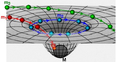 |
A material gravitational body curves
space-time in its vicinity (example of a spherically symmetric body) |
In our terrestrial gravity conditions, it can be clearly illustrated by horizontally tensioned flexible curtain (which represents not curved space without gravity), on which lay the material sphere M. The recess created by the load represents the curvature of the space. When we place a smaller ball m1 (rest) here, will roll into a depression and lands on a larger ball. However, if we give the ball m2 a suitable circumferential speed, it will orbit a heavy sphere, which is the source of curvature, much like a planet orbits a gravitational star or a moon-satellite around a planet. At a higher ball speed m3, its path in the recess only curves and the ball continues to move at a different angle.
The local differential
equations of field excitation express the global integral
behavior of the field
In field theory, the laws of its excitation by
their sources, as well as its internal dynamic properties, are
expressed by means of differential equations.
These equations have a local character - they
relate the local distribution of matter or
electric charges with the derivatives of the field intensity or
the curvature of spacetime in the same place.
However, this does not mean that the sources determine the values
of the quantities describing the field only locally or in the
immediate vicinity of the field sources. By integrating
the local differential equations of the field, we obtain the
values of the field intensity or the curvature of spacetime in
the whole space surrounding the source system.
This happens so often through boundary conditions,
as we will see, for example, in §3.4 "Schwarzschild
geometry".
The equations of motion of
resources as a consequence of the field equations
Covariant 4-divergence left part G ik Einstein's equations (2.50) is
identically equal to zero. This is due Bianchi identities (2.25)
for the curvature tensor, a manifestation of the principle of
geometric-topological "boundaries boundary equals zero"
- in this case the oriented two-dimensional boundary of the
three-dimensional boundary of the four-dimensional region of
space [180] [181] (see also §3.1 "Geometrical
-topological properties of spacetime").
Therefore, if we take Einstein equations (2.50) as a basis, it
follows them automatically Tik;k = 0 - the local law of
conservation of energy and momentum of the source *). This law of
conservation leads to the equations of motion of the source
system described by the corresponding energy-momentum tensor Tik , so in this sense "the equations of motion flow from the Einstein
equations of the gravitational field ". Einstein gravitation
equation thus determine not only the gravitational field for a
given mass distribution, but they also determine the motion of
this source.
*) It is an expression of the
general regularity between the source and the field it evokes:
"the source creates a field around itself so
that it preserves itself "
- the field of such properties, from which the conservation
laws of this source
automatically follow. E.g. for the electromagnetic field from the
Maxwell equations Fik ; k
= 4p j i/c due
to the antisymetry of the electromagnetic field tensor Fik, the relation j i ;
i = 0 follows
identically, which is the equation of current continuity, i.e.
the law of conservation of electric charge. Maxwell's equations
thus limit the "freedom" of resources only in terms of
electrical (not eg mechanical), while Einstein's gravitational
equations affect all forms of resource motion.
Unlike all other field theories, the
general theory of relativity has the specific property that it is
not necessary to postulate separately (enter "from
outside") equation the motion of test particles in a given
gravitational field - these equations of motion can be obtained
as a consequence of the field equations. Indeed, the application
of the law of conservation of energy and momentum (2.6) of a test
particle, resulting from Einstein's equations (2.50a), leads to
its geodetic motion [78] described by equation
(2.5). Gravity and mechanics are inextricably linked
("unification of gravity and mechanics") in contrast to
Newton's theory, where they are completely independent.
Similarly, if we have a free electromagnetic field in a vacuum,
then from the Einstein equations (on the
right side of which is the energy-momentum tensor of the
electromagnetic field) of the gravitational field excited by this
electromagnetic field, result the Maxwell's equations Fik
; k = 0 of free electromagnetic field; an
interesting interpretation of this fact for unitary field theory is in the geometrodynamics of
Wheeler and Misner, see Appendix B, §B.3 "Wheeler's
Geodynamics. Gravity and Topology.".
Solving Einstein's
equations
Let us now turn to the question of how to determine the structure
of spacetime in given physical situations, ie how to solve Einstein's gravitational equations. The
straightforward use of Einstein's equations to determine the
evolution of a physical system based on suitable initial
conditions - the so-called Cauchy
problem - will be outlined in §3.3 "Cauchy
problem, causation and horizons". Einstein's gravitational
equations (2.50) are tensor nonlinear partial differential
equations of second order, so their general solution is very
difficult and in most cases can not be found analytically. There
are several ways to simplify the solution :
Weak gravitational field - linearized theory
of gravity
Appropriate approximations of the general theory of relativity -
the so-called linearized theory of
gravity -
can be used for weak gravitational fields. In the linearized theory of gravity, Einstein's equation and equation of motion
are formulated and solved as if spacetime is substantially
planar, with only a very small curvature characterizing gravitational
phenomena. For sufficiently weak fields and in a suitable (almost
inertial) frame of reference, the metric tensor can be expressed
in the form
| gik = hik + hik ; | hik | << 1 , | (2.51) |
where hik is the Minkowski flat space-time
tensor and hik is a small
"correction" expressing a weak gravitational field. The
components hik are proportional to the
Newtonian gravitational potential, as we determined for hoo in §2.4, relation (2.27), and for the
other components h we find it below.
We then decompose the nonlinear Einstein's
gravitational equations in a series according to the powers hik, and due to their smallness we can neglect
their products and powers without much loss of accuracy and leave
only the members of the first order; thus we get the sought linearized equations. Linearized connection coefficients for
metric (2.51) are Gi kl = (1/2) (hik, l + hil, k - h, ikl) and Ricci's curvature tensor with 1st
order precision in hik has the form Rik = (1/2) (hl i,
kl + hl k, il - hl ik,
l - h, ik), where h ş hi i = hik hik; while the indices at hik are "raised" and
"triggered" by hik , not the whole gik (contributions from hik they are second order and neglected).
Einstein's equations in this approximation are then
hil,kl + hkl,il - hik,ll - h,ik - hik(hlm,lm - h,ll) = (16pG/c4) . Tik .
If we introduce quantities
| yik = hik - 1/2 hik h , | (2.52) |
these equations have the form
- yik,ll - hikylm,lm + yil,kl + yik,ll = (16pG/c4) . Tik .
One can show that, without loss of generality it is possible for the variable yik introduce calibration - gauge conditions *) [271]
| yik, k = 0 | (2.53) |
analogous to Lorentz
gauge conditions Aik, k = 0 in electrodynamics.
*) The procedure of gauge
transformation in field theory is generally discussed in
§B.6, passage "Calibration - gauge
- transformation; calibration - gauge - field".
The linearized Einstein equations then take on a simple form
| - yik,ll ş o yik = (16p G/c4) . Tik , | (2.54) |
where oş ¶2/¶x2 - (1/c2) ¶2/¶t2 is the d'Alembert operator. The general solution of these linearized gravitational equations in Lorentz gauge (2.53) can be expressed in the form of retarded potentials
| (2.55) |
similarly to electrodynamics, where R = Ö[a = 1S3 (xa - x'a)2] is the distance from individual places x'a the source system to the investigated point xa (similar to Fig.1.4a). The retarded solution (2.55) shows that changes in the gravitational field propagate at the speed of light. The significance of this solution for gravitational waves will be discussed in §2.7 "Gravitational waves" (where in the passage "How fast is gravity?", general questions of the speed of propagation of changes in the gravitational field will be briefly discussed).
Here we will consider a situation where the gravitational field is excited by a source for which Newtonian physics applies with sufficient accuracy, ie the velocities are small and Too << |Ti a|. Moreover, if found close enough to the source, or if the resource is static (i.e. we located in the "inductive" zone r << c.T, where T is a characteristic time changes in the distribution of mass in the source), retardation can be neglected and solution (2.55 ) has the form
yoo = - 4j/c4 , yoa = 0 , yab = 0 ,
where j(t,xa) = -G.ň(Too(t,x'a)/R)dx'1dx'2dx'3 is the ordinary Newton's potential. In this case, the metric (2.51) is
| ds2 » - c2(1 + 2j/c2)dt2 + (1- 2j/c2)(dx2+dy2+dz2) , | (2.56a) |
i.e.
|
The expression (2.27) for the time component of the metric tensor for weak fields is thus supplemented by other components. At distances r substantially greater than the dimensions of the source, R»r can be approximately lay down and the metric (2.56a) can be expressed by the total mass M = ň T°° d3x of the source system :
| (2.56c) |
This metric is an approximate expression of the Schwarzschild geometry (3.13) derived in §3.4 "Schwarzschild geometry".
Rotating gravity
In the more general case, when the velocities at the source of
the gravitational field can be large and the components of the
stress tensor Tab and the momentum density T°a can be comparable to the mass-energy
density T°°, a weak gravitational field at a sufficient
distance from the source can be approximately determine by
distributing the retarded potentials (2.55) into a Taylor series
according to the powers of x'/R. In the rest frame of reference
with the origin in the center of gravity (ie Pa = ňT°ad3x = 0, ňxaT°°d3x = 0) then after suitable gauge
we get with an accuracy of 1/r :
| (2.56d) |
where Ja = ňeabgxbTg°d3x is the
intrinsic (rotational)
angular momentum of the source body.
Gravitational-wave members in metrics we
will not be analyzed here, their meaning and properties will be
discussed in §2.7 "Gravitational
waves".
Here we will mention some gravidynamic
effects.
In polar coordinates with the polar axis oriented in the
direction of the angular momentum vector J, the external gravitational
field of the rotating body will be described by an approximate
metric
| (2.56e) |
which is a special case
of general Kerr geometry
(3.37) for a small angular momentum J (§3.6 "Kerr and Kerr-Newman geometry").
In
Newton's theory, the gravitational field is given only by the
distribution of matter and does not depend at all on the
instantaneous velocity of individual parts of the source or on
its possible rotation (unless, however, it leads to changes in
the mass distribution). In GTR, however, the rotation of the source leaves characteristic
"traces" on the external gravitational field (ie on the
space-time metric) in the form of non-diagonal members *) .
*) This metric cannot be
diagonalised without the explicit dependence of the components of
the metric tensor on the time t .
These off-diagonal
members dj.dt lead to the effect, that a certain
additional force acts on the bodies (in the geodesic equation the
d2j/dt2 ą 0 becomes non-zero), which causes
entrainment of the local inertial
system ( frame
dragging) - entrainment of free bodies by a rotating
gravitational field in the direction of rotation of the source.
It is similar to a sphere rotating in a viscous liquid, which
drivess the liquid near its surface into rotation. This
phenomenon is called the Lense-Thirring
effect
according to the authors who first studied it [248]. For
common rotating bodies (macroscopic objects, planets, ordinary stars, etc.) the effect of entrainment is
very small, but it can be crucial for rotating
black holes
(in accretion disks and especially in the so-called ergosphere), as will be shown in §4.4 "Rotating and electrically charged Kerr-Newman
black holes".
 |
Hydrodynamic analogy of the
influence of the rotation of the source body on the
properties of the excited gravitational field. Left: In Newton's theory, the gravitational field of a body is given only by the distribution of matter and does not depend at all on its possible rotation (unless it leads to changes in the distribution of matter). Similarly, a smooth and symmetrical body (such as a sphere) rotating in an ideal liquid without viscosity does not cause the liquid to move around it. Right: In the general theory of relativity, however, the rotation of the source leaves characteristic "traces" on the external gravitational field (on the space-time metric) - local inertial systems are entrained - free bodies are entrained by the rotating gravitational field in the direction of the source rotation. Similarly, a body rotating in a viscous liquid entrains the liquid near its surface into rotation. |
Magnetogravity -
gravitoelectromagnetism ?
For these gravidynamic effects, a certain analogy can be traced with magnetism in electrodynamics. In §1.4 "Analogy
between gravity and electrostatics" we have shown that the
Newtonian gravitational field is, from the formal point of view
of the mathematical description, completely analogous to the
electric field. More generally, it can be shown that there are formal analogies between the equations of electromagnetism
(Maxwell's equations) and special approximations of Einstein's
gravitational equations in GTR. This analogy is sometimes
referred to as gravitoelectromagnetism - some specific kinematic
effects of gravity are analogous to the magnetic effects of
moving charges. This is mainly the above-mentioned effect of entraining bodies in the direction of rotation
of the source of the
gravitational field (Lense-Thirring
effect), which
is somewhat reminiscent of magnetism. Using special
"purpose" transformations, Einstein's gravitational
equations can be modified into the form of electromagnetism
equations.
From an objective point of view, however,
these analogies are only formal, with little physical
significance. Phenomena seemingly reminiscent of magnetism are of
the second and higher order in comparison with the primary
gravitational ("gravistatic") action. Real physical magnetism caused by the interaction of moving
"charges" - the sources of field - is not contained in gravity ...
Note 1: For
the magnetism of gravity could be considered well-known Coriolis
force Fc = -2 m. [v x w], which resemble the magnetic Lorentz force Fm = (1/c) .q. [v
x B] applied
perpendicularly with electric charge q moving speed v in
the magnetic field intensity (induction) B.
However, these forces are in fact only a kinematic effect in
a rotating frame of reference (angular velocity w),
occurring even in classical Newtonian mechanics ...
In the field of electricity,
magnetic phenomena are well manifested in normal
laboratory conditions because the electric force effects of
positive and negative electric charges are annulled on average,
so they do not overlap dynamic magnetic effects. A metal wire
(conductor) is generally electrically neutral even when a stream
of charged electrons passes through it; the resulting magnetic
field can thus exert an undisturbed force on the second (also
uncharged) conductor with an electric current.
In the field of gravity, however, the attractive
"gravistatic" forces add up, so that in this strong
static field, the subtle gravidynamic effects
are normally completely everlaid by static
gravity. Ordinary macroscopic bodies, planets and stars can never
move or rotate at high (relativistic) speeds in bound systems, so
they can excite strong gravity, but only minimal dynamic effects.
Only in compact gravitationally collapsed objects, neutron stars
and especially black holes, the rotational
motion can be relativistic, as a result of which gravidynamic
effects can almost equal gravitational forces and can manifest
significant astrophysical effects - §4.4 "Rotating
and electrically charged Kerr-Newman black holes" and §4.8 "Astrophysical significance of
black holes".
Note
2: In
this context, we can also mention analogy of
electromagnetic and gravitational waves - §2.7 " Gravitational
waves ". It is also
interesting to note that even in "empty" space without
material sources, a source of the global gravitational field
appears on the right-hand side of Einstein's equations - Isaacson's
tensor of "effective distributed" energy-momentum
of gravitational waves (2.76). This is somewhat analogous to how
the Maxwell shear current (cf.
§1.5, equation (1.34)) excites the magnetic field as well as the
current of real electric charges, even in a vacuum without
currents for a non-stationary electromagnetic field. However,
even this analogy is formal, without a direct connection with
magnetism ...
Thus,
it cannot be expected, that gravidynamic
phenomena could allow, even in principle, some "gravitronics"
- the gravitational equivalent of electronics on a cosmic scale!
Possibilities
of verification of the effects of rotation
Despite the very small effect of rotation on the excited
gravitational field, however, in the 1960s several experts from
the University of Stanford (L.Schiff,
G.Pugh, R Conannon, W.Fairbank, F.Everitt, N.Roman) proposed, but for a long time not
performed *), highly sensitive experiments
that could demonstrate this effect and measure even in the weak
gravitational field of the Earth by accurately monitoring changes in the direction of the rotational axis
of the gyroscope - precession, orbiting in polar orbit. The
rotation axis of such flywheel will change during orbit due to
two GTR effects :
a) The gyroscope orbits in the curved
spacetime of the Earth's gravitational field - geodetic effect,
connections, change of vector direction during parallel
transmission - see §2.4. This effect geodetic
precession
should be dominant and lead to a change in the axis of rotation
in the direction of movement of the probe in orbit by about
6''/year.
b) Due to the entrainment by the Earth's
rotational angular momentum, the rotational axis of the gyroscope
should show a slight "anomalous" precession - twisting
in the Earth's direction of rotation (for a polar orbit
perpendicular to the plane of orbit) at an angular velocity
proportional to the Earth's angular momentum and indirectly
proportional to the cube of the orbital radius. The expected
value of this anomalous Lense-Thirring
precession is
only a few hundredths of an angular second per year (approx.
0.04''/year for the proposed orbit approx. 600 km above the
Earth).
Both of these deviations a), b) are
perpendicular to each other. To objectively demonstrate the
effect, it is necessary to compare the rotational axes of at
least two gyroscopes rotating in opposite directions.
Another possibility is an
accurate analysis of the orbit of special satellites **) and an
analysis of the orbital dynamics of tight binary pulsars ***).
*) Gravity Probe B
This experiment was at the project stage for a long time. After
overcoming a number of technical difficulties and long-term
testing (team led by F.Everitt), the Gravity Probe B
satellite was launched on April 20, 2004 , in o polar orbit at a
height of 640 km, which carried 4 precision gyroscopes with a
diameter of 3.8 cm, rotating at a speed of 10,000 rpm. Two rotate
in one direction, two in the opposite. Their surface is coated
with a superconducting layer of niobium. During its rotation,
this superconducting layer generates a magnetic field, which is
monitored by electromagnetic induction in the so-called SQUID
(Superconducting QUantum Interference Device) electronic device,
which with high sensitivity (10-4'') detects the deviation of the axis of rotation of the
gyroscope. The case with the gyroscopes is connected to a small
pointing telescope focused on the star IM Pegasi, which ensures
the reference direction of the rotational axes of the gyroscopes.
To increase the sensitivity of the measurement (signal-to-noise
ratio), the entire measuring system is built inside a Dewar
vessel with 2400 liters of liquid helium, which cools the
measuring box to 1.8 °K during an operating time of more than
1.5 year. Data transmitted by the satellite were collected
until February 2006.
The high sensitivity of the installed
equipment gave hope that during the planned approximately 18
months of measurements, the peculiar very fine dynamic-kinematic
effects of the general theory of relativity will be verified with
high accuracy. During operation the Gravity Probe B , encoutered
difficulties. Disorders from the solar protuberances caused
disturbing deviations in the positions of the rotational axes of
the gyroscopes, and other noises appeared. From the native data
it was not possible to accurately prove the analyzed effects
(especially the Lense-Thirring effect). The whole two years took
a complicated processing of results - data filtering and removal
of various types of faults and noise. The resulting measured
values after this treatment were finally: geodetic precession
(6601.1 ± 18.3) x10-3
''/year, compared to the GTR predicted value 6606.1x10-3
''/year; Lense-Thirring precession (37.2 ± 7.2) x10-3
''/year, compared to the GTR predicted value of 39.2x10⁻³
''/year. However, the excessive complexity of data processing
somewhat reduced the validity of the results ..?..
**) Satellite orbit analysis
Both of these subtle "gravidynamic" GTR effects can
also be detected with comparable accuracy by measuring the orbit
of the Laser Geodynamics Satellite (LAGEOS). This satellite
consists of a metal sphere with a diameter of 60 cm, equipped
with 426 passive laser mirror reflectors (so-called
retro-reflectors). It orbits the Earth in low orbit at an
altitude of 5,900 km. Measurements are made using reflections of
laser pulses from many ground stations - the time intervals
between sending the beam and receiving the reflected pulse are
evaluated, which allows you to measure instantaneous distances
very accurately. These measurements of the exact positions of the
satellite relative to different places on the earth's surface
make it possible to measure the shape of the earth's geoid and to
study the movements of tectonic plates and terrestrial
continents.
However, by measuring the
differences between the orbits of many successive orbits, the
contribution of the Lense-Thirring effect - the relativistic
precession caused by the rotational angular momentum of the
Earth's - can also be determined here. This gravitomagnetic
action will change the point of the closest approach of the
satellite to the Earth (perigee) by about 3 meters / year.
However, there are a number of disturbing influences such as the
pressure of solar radiation, the gravitational action of the
Moon, tides, geological inhomogeneities, ....
***) Dynamics of binary pulsars
Another possibility is the observation of binary pulsars, here
especially PSR J0737 + 3039 and PSR J1757-1854. These two
orbiting neutron stars are rapidly rotating massive compact
objects at a short distance from each other in a massive
gravitational field, so that all generally relativistic effects
are much stronger here than in the faint gravitational field
around Earth. Measurement of the periastron shift in relation to
the moment of inertia of the double pulsar can assess the
contribution of the Lense-Thirring effect (gravito-magnetic
spin-orbital precession of the periaston). ....... .......
Three
aspects of space-time curvature
In the general theory of relativity, thus there are three basic
ways of space-time curvature due to different
mass-energy distribution and its temporal dynamics :
× Space
curvature
× Time deformation
× Rotational motion of space
Do
material bodies create space and time ?
The cause (essence) of gravity in the general theory of
relativity is the geometric properties - curvature - of
spacetime. And this curvature of spacetime is generated by
material bodies. The implications [material bodies -> gravity
-> spacetime] are sometimes shortened and simplified by the
formulation that "bodies create spacetime",
"spacetime is an integral part of bodies".
From there, it is only a step to the claim "without
material bodies there would be no space and time",
which is sometimes mentioned in the interpretation of the general
theory of relativity. However, this claim is already misleading!
Einstein's equations (2.50) have a planar spacetime in empty
space without the presence of material bodies as a simple
solution of Minkowski flat spacetime, in which the test particles
move according to the laws of a special theory of relativity. And
at the early stages of the evolution of the universe, when there
were no bodies (and initially no particles
or particular fields), existed here
a rapidly expanding space from which our later universe
came into being (§5.4 "Standard
Cosmological Model. The Big Bang. Shaping the Structure of the
Universe."). Only at the very origin of the universe ("big bang"), the
standard cosmological model does assume, that space and time
were also created here, which "did not exist"
before... - §5.4, passage "The
beginning of time?".
Thus, in interpreting and discussing the general
theory of relativity, we would recommend not using
the misleading statement that "material bodies create
spacetime", but only a physically justified formulation
that "material bodies curve spacetime around
them". And not only material bodies, but also
physical fields...
Note: From a philosophical-gnoseologic point of view, however,
it is possible to discuss whether without the existence of
particles or bodies the terms space and time have real
meaning..?.. We should not measure "by what" neither
"nothing real" ...
Variational Derivation of Einstein's Equations of
the Gravitational Field
The culmination of the mathematical structure of every physical theory is the
formulation of its laws using Hamilton's variational principle
of least action [165], [166]. This approach consists in
constructing a Lagrange function
(Lagrangian) L
for the investigated physical system, such that its integral - action - is extreme for real motion (trajectory,
evolution), ie the variation of the action is zero. From this
then follows the basic Lagrange
equations of motion of a given physical systems. The main benefit
of the variational method is that it helps to clarify some
structural laws of the theory, such as the relationship between
the principles of symmetry and conservation laws, the uniqueness
of equations of motion and the like.
For the system [source
bodies + excited field], the total quantity of the action can be
considered as the sum of three terms: S = Sm + Sf + Smf , where Sm is the action of the source
bodies (particles), Sf is the action of the field
itself and Smf expresses the mutual interaction
of particles with the field. For a physical field in the theory
of relativity, the action is given by the integral of the
Lagrangian Lf , which is a function of the
field potentials and their derivatives over the investigated
4-dimensional spacetime region W: Sf
= ň Lf (j, j, i) dW , d W = dtdxdydz. In relativistic
physics, it is also advantageous to write the quantities Sm
and Smf in the form of integrals (Sm
= ň Lm dW over
a 4-dimensional space-time region), ie to use the approach of
continuum physics. When determining the
possible shapes of the Lagrangian, resp. integral of the action,
is based on certain general physical requirements for the
resulting field equations, such as relativistic invariance (general
covariance), resp. linearity (superposition principle), symmetry,
the degree and the like. From the group of
possible Lagrangians thus defined, it is then often selected
according to "aesthetic" criteria of simplicity.
For example, for an electromagnetic field,
the described vectors of electric and magnetic field intensities,
it follows from the requirement of linearity of field equations
(superposition principle) that the Lagrangian must be a quadratic
function of the field intensities; the simplest scalar
(relativistic invariance) of these properties, created
from components of electric and magnetic intensities, is the
summation product Fik Fik of the electromagnetic field
tensor component (1.114), so the integral of the action for the
electromagnetic field has the form Se = k. ň Fik Fik dW. The
total Lagrangian of the charged particle system and the
electromagnetic field is then [166] L = -rmc2 + (1/16pc) FikFik + (1/c2)Aij i . From the variational principle
dS = d ňL dW = 0, then we can get both the
equations of motion of particles in the electromagnetic field (if
the electromagnetic field is considered as a given and varying
the particle trajectories), and Maxwell's equations of
electromagnetic field (while varying the 4-potential
components at the specified distribution and movement of
charges).
For the gravitational field in GTR, when
the investigated physical system consists of a system of source
(material) bodies and an excited gravitational field, the total
action will be given by the sum of S = Sm + Sg, where Sm= ňLm(qa,qa,i)Ö(-g)
dW is the integral of the action of the
source part described by the generalized coordinates qa
(a = 1,2, ..., N is serial number of the generalized coordinate)
and Sg= ňLg(gik)Ö(-g)
dW is the action of the gravitational field
itself described by the components of the metric tensor gik. The factor Ö(-g)
comes from curvilinear coordinates - it guarantees that the
product Ö(-g) dW behaves as an invariant when integrated
over a 4-dimensional volume. The interaction term is not here,
because it is implicitly contained in the term Sm
(by describing the source by physical laws in the curvilinear
coordinates of curved spacetime, its interaction with the
gravitational field is also expressed). The Lagrangian Lg
must be a scalar function of the metric tensor gik and its derivative, so that the
variations of the resulting field equation contain derivatives
not higher than the 1st order. The simples such scalar is a
scalar curvature R spacetime (2.24); if we also
admit the presence of the constant term C = const., the
Lagrangian of the gravitational field could have the shape Lg
= k.R + C. In order to obtain the Einstein equation directly with
the usual form of constant factors, writes this Lagrangian in the
form Lg = (c3/8p G)
(R - 2 .L ), where G is Newton's
gravitational constant and L is the cosmological s constant.
The variation principle dS = d (Sg
+ Sm) = 0 at complete variation then after
adjustments gives the relation [166]
is a tensor of energy - momentum of a source. The variation of the metric gik gives Einstein's equations of the gravitational field
Rik - (1/2) gikR - L.gik = (8pG/c4) Tik ,
while the variation of the source variables qa leads to the equations of motion of the source system (non-gravitational fields):
![]()
A brief recap and
reflection on gravity :
Effect and nature of gravity
Gravity is one of the 4 basic forces of nature, it is responsible
for the attraction between all material objects in the universe.
In classical physics, the gravitational force between bodies is
described by Newton's law of gravity (§2.1), which works perfectly in all situations that we
practically encounter here on Earth and in the planetary Solar
System. That is, with relatively weak gravity and slow speeds of
movement of gravitating bodies.
Within the modern physics of gravity, which also
generalizes it to strong gravitational fields and high
speeds of movement - Einstein's general theory of
relativity GTR - gravity is described as a curvature
of spacetime, caused by matter (and energy). Material
objects such as planets or stars cause geometric deformation
- the curvature of spacetime around them. This curvature is also
caused by physical fields such as electromagnetic radiation (ie also light). Other surrounding
objects, such as planets (even those light
rays, photons), in their free movement,
"free fall", naturally follow curved paths, so-called geodesics,
in this curved space-time. This gives the impression of gravitational
attraction: when surrounding bodies move along these curved
paths, they appear to be attracted by the massive object that
caused the curvature of spacetime.
Thus, according to general relativity, gravity is
not a force in the traditional sense, such as the
electromagnetic or strong nuclear force. Here it is a consequence
of the deformation - curvature - of space-time caused by
material objects. Other objects then move in this curved
space-time along paths dictated by the curvature, giving
rise to the gravitational force as we perceive it...
It is also interesting to consider the different
role of the geometric curvature of 3-dimensional space and
the "curvature" of time (different
speed of time flow) in GTR - it is
discussed in the previous §2.4, the final passage "What gravitates more - curved space or
curved time?".
Is gravity really just curved spacetime ?
In the previous §2.1-2.4, we showed that within the theory of
relativity, according to the principle of equivalence of
gravitational and inertial forces, gravitational action can be
described as an effect of the curvature of spacetime.
General relativity states that gravity is curved spacetime (we
also use this concept throughout this book "Gravity, Black
Holes..."). But the question is
whether such a complete identification is not too strong
a statement from an epistemological point of view..?.. Whether
the geometric curvature of space-time is not just a model
consequence of gravitational action, albeit the most
important one. Perhaps it would be sufficient to formulate that gravity
curves spacetime, while this curvature is universally
excited by all mass~energy according to Einstein's gravitational
field equations (2.50) in GTR..?.. Or that gravity in GTR is
modeled geometrically - by curved spacetime..?.. Keep in
mind that it is only a mathematical model of
physical reality, albeit a very successful one !
General theory of relativity and the
nature of gravity
The question of whether the general theory of relativity explains
the essence of gravity cannot be answered other than: yes and no ! The general theory of relativity
converted gravitational action into inertial motion - it merged
gravity and inertia, identifying them with the geometric
properties of spacetime. It converts the laws that govern gravity
into the laws that govern space-time. Thus, unifying
relationships between previously separated phenomena were
discovered. To the question of the cause of
gravitational action, the general theory of relativity answers
with curved spacetime, but does it not explain why bodies in their surroundings curve
spacetime? The general theory of relativity shows how, but not why. The only complete answer - but from the opposite side - could perhaps be given by a
consistent unitary field theory (see the individual chapters of Appendix B "Unitary
Field Theory"): that bodies and particles of
matter are local "condensations"
of curved empty spacetime....
But the deepest primal foundation of "why?"
and "how next?" we probably don't
explore so far..?..
| Gravity, black holes and space-time physics : | ||
| Gravity in physics | General theory of relativity | Geometry and topology |
| Black holes | Relativistic cosmology | Unitary field theory |
| Anthropic principle or cosmic God | ||
| Nuclear physics and physics of ionizing radiation | ||
| AstroNuclPhysics ® Nuclear Physics - Astrophysics - Cosmology - Philosophy | ||