| (2.5b) |
| AstroNuclPhysics ® Nuclear Physics - Astrophysics - Cosmology - Philosophy | Gravity, black holes and physics |
Chapter 2
GENERAL THEORY OF
RELATIVITY
- PHYSICS OF GRAVITY
2.1. Acceleration and gravity from the point
of view of special theory of relativity
2.2. Versatility
- a basic property and the key to understanding the nature of
gravity
2.3. The
local principle of equivalence and its consequences
2.4. Physical laws in curved spacetime
2.5. Einstein's
equations of the gravitational field
2.6. Deviation
and focus of geodesics
2.7. Gravitational
waves
2.8. Specific
properties of gravitational energy
2.9.Geometrodynamic system of units
2.10. Experimental
verification of the theory of relativity and gravity
2.4. Physical Laws in
Curved Spacetime
Gravity can
be examine in essentially two ways :
Either:
1. Consider
a "physical" gravitational
field in
planar spacetime (within STR) ;
And or:
2.
Introduce curved spacetime without gravity .
In the first mode, we consider the
universality of the gravitational interaction to be a coincidence, but its consistent application in the
equations of the gravitational field ultimately leads to
nonlinear Einstein equations and the need generalization of the special
theory of relativity, as mentioned in §2.1. The second approach,
which from the very beginning draws appropriate consequences from
the universality of gravitational action, identifies the
gravitational field with the geometric properties of spacetime.
The gravitational force is the result of "deepening"
and distortion in the cosmic structure of space and time.
The implementation of this procedure is
actually the content of the general theory of relativity.
According to Newton's classical physics, planets orbit the Sun in
a circular (elliptical) orbit because they are immediately
attracted to it by gravitational force, which causes a centripetal
acceleration, curving orbits that would otherwise be straight.
According to the general theory of relativity, however, between
the Sun and planets no gravitational
forces acts - the orbits of the planets are
curved because the actual space and time in which they move is
deformed (curved) by the presence of the massive Sun and
automatically forces the planets to move along the respective
"geodetic" orbit.
In terms of general relativity, the
movement of the test particles in a gravitational field is inertial (particle is free) and its possible
peculiarities are caused not by the "gravitational
force" acting on the particle, but by the space-time
metric; it
is similar with all physical phenomena in the presence of
gravity.
The gravitational field thus
"disappeared", instead of him the generally curved (Riemannian) spacetime here remained. And the problem
of finding the physical laws governing natural phenomena in the
gravitational field thus translates into the question of
determining the physical laws in the curved Riemann spacetime
(without gravity).
Using the principle of equivalence, it is possible to generalize all the physical laws of the special theory of relativity (where the Minkowski spacetime is planar) to curved spacetime, ie to the presence of a gravitational field. The method described in the previous paragraph leads to a straightforward approach: to divide spacetime into sufficiently small areas in which the curvature can be neglected, to apply physical laws spacetime in these areas (ie STR formulated for general reference frames) and finally to fold this of planar "mosaic" in the resulting global situation.
We can illustrate this general procedure with simple examples. Consider a test particle (mass m , which are not explicitly not applied) moving in a given gravitational field, which at time t is in world-point P. If we introduce at point P a locally inertial reference system S~ with Cartesian space-time coordinates x~ i related to the owen time t of the test particle by the relation dt2 = - (1/c2) hik dx~ i dx~ k, there will be a "weightlessness" state without gravity field in this system at time t in the vicinity of the test particle, and a special theory of relativity will apply locally. The equations of motion of the test particle in this locally inertial system will therefore be (uniform rectilinear motion)
| d 2 x ~ i / d t 2 = 0 . | (2.5a) |
If we go as in §2.1 from the system S~ to the general non-inertial frame of reference S with space-time coordinates x i related to the own time by the relation
ds2 = - c2dt2 = gik dxi dxk ; gik(x j) = hlm.(¶x~l/¶xi).(¶x~m/¶xk) ,
the equation of motion (2.5a) is transformed into the form of the geodetic equation
| (2.5b) |
wherein Gkil = (1/2) gim (¶gmk/¶xl + ¶gml/¶xk
+ ¶gkl/¶xm) as shown in §2.1, equation
(2.2a,b). We can do this procedure at any point of a test
particle world-lines and we always get the equation of shape
(2.5b). Equation (2.5b) is thus the general
equation of motion of a test particle in a gravitational field
(in curved spacetime), which is invariant (covariant) with respect to any
transformation of spacetime coordinates. Here, this equation of
geodesy serves only as an example of the general procedure of
finding the laws of physics in the presence of gravity; we will
return to its physical significance below.
As a second example, we take the
differential law of conservation of
energy and momentum, which has in the form Tik, k ş ¶Tik/¶xk = 0 in STR (see §1.6). It will
have the same wording in every locally inertial frame of
reference S~ moving freely in a gravitational
field: ¶Tik(x~)/¶x~ k = 0. After transformation into a
general (non-inertial) frame of reference S, this law takes on a covariant
form
| ¶Tik/¶xk + Gmik Tmk + Gmkk Tim = 0 , | (2.6) |
which represents the
formulation of the law of conservation of energy and momentum in
curved spacetime, ie in the gravitational field. The physical
aspects of this law will again be discussed below (in §2.8).
From these two cases we can already deduce
general laws. According to the principle of equivalence, the
physical laws in the gravitational field are locally the same as
the physical laws in non-inertial frame of reference without
gravity. The non-inertial frame of reference is then
mathematically equivalent to a curvilinear system of space-time
coordinates. Thus, it can be expected that the generalization of
physical laws to the presence of a gravitational field (ie their
formulation in curved spacetime) will simply consist in writing
these laws in general curvilinear
coordinates.
The difference compared to the planar spacetime (situation
without gravity) is then only that that in the flat spacetime can
be by suitable transformations always return to the laws of
special theory relativity in Cartesian global inertial system,
while for the curved spacetime this is not possible, the global
inertial system here does not exist, there are only
"curvilinear" coordinates.
Parallel
transfer of vectors, connections, covariant derivation
Physics studies the course of natural processes in different places in space and in different times -
at different points in space-time. It describes the physical
processes by the relevant physical quantities in these places,
which leads to certain physical
fields. In
common situations of Euclidean space, or Minkowski spacetime, we
do not have to worry about the differences in the geometric
properties of space in different places - these are identical
Euclidean (or pseudoeuclidean). However, in the general theory
of relativity, which implies more complex geometric properties of
curved spacetime, non-trivial relationships arise between
different places in space and time, which can affect the values
of physical fields. These relationships between quantities at
different points in space (and spacetime) are quantified by the
geometric-topological concept of connection
(from the Latin connectio =
connection, intercourse, binding). The
connection analyzes what needs to be done with the values of the
components of the vectors and tensors describing the physical
field - what correction to make to express the objective
values of the fields, independent of
the local geometric conditions and the coordinate system used.
The laws of physics are expressed by
differential equations between vector and tensor fields in spacetime. Ordinary partial derivative
of vector field Ai according to coordinates xk
| (2.7) |
is usually a measure of how the vector field Ai changes with location (from a
point with xk coordinates to a
"neighboring" point xk + Dxk).
However, when using curvilinear coordinates for objectively
comparing vectors and tensors entered at different points in
spacetime, their components calculated with respect to the local
base cannot be used immediately, as they may be different at
different points. The components of vectors and tensors (vector
and tensor fields) can change from point to point using
curvilinear coordinates for two reasons :
a ) First,
because a given vector field actually (physically) changes with
place.
b ) Furthermore, also because there
is a different vector base in each place, with respect to which
the components of vectors and tensors are determined - this can
lead to different values.
Normal partial derivatives of (2.7) are
then objectively not actual changes in vector and tensor fields,
as e.g. also constant vector field will have to curvilinear coordinates variable components, and
therefore a non-zero partial derivatives of its components. In
addition, Ai , k is not
transformed as a tensor, because the difference between the
vectors Ai is at different points where there
may be different transformation coefficients.
An appropriate correction to these circumstances must be
made - take into account the connection: first transfer the vectors in
parallel to one common point and then compare their
components. At parallel transfer vector, its components in the
Cartesian coordinate system not changes. Using a curvilinear coordinate
system, however, when parallel transfer vector Ai
from the point with coordinates xk to a nearby point xk
+ Dxk components of the vector changes
by
| d A i = - Gk i l A l . D x k , | (2.8) |
where the quantities Gk i l (which depend on the coordinate system) are the Christoffel coefficients of the affine connection, which we have already encountered in §2.1, relation (2.2b). It is clear that the quantities G k i l cannot form a tensor, because by transitioning from the Cartesian system, where they are all equal to zero, to the curvilinear system they become nonzero (and vice versa, with nonzero Gk i l , all components can be canceled by going to the Cartesian system at a given point). From the requirement, that dAi in the law of parallel transmission (2.8) be transformed as a vector, for affine connection coefficients follows the transformation relation :
| (2.9) |
From this it can be seen
that the connection coefficients behave as tensors only in linear
coordinate transformations (such as transformations between
Cartesian coordinate systems).
The resulting components of the vector Ai(xk) transferred in parallel to the
point xk + Dxk will be Ai(xk)®xk+Dxk = Ai(xk) + dAi. The requirement that the rules
of tensor algebra be preserved during parallel transfer, follows
from (2.8) for the parallel transfer of the general tensor T irjs....... the law :
| d T irjs.......
= - Gmin T mrjs........Dxn
- Gmin T irms........Dxn
- .... + Grmn T imjs........Dxn + Gsmn T irjm........Dxn + .... . |
(2.10) |
The "correction" of the partial derivative (2.7) to the change of the vector base caused by the "curvature" of the coordinates then consists in the fact that during the derivation the parallel transfer of the vector Ai(xk + Dxk) from the point xk + Dxk back to point xk is performed, and only then the appropriate limit be made :
| (2.11) |
It is thus achieved that is taken the difference between the components of the vectors calculated at a single point xk, and thus related to the same base. This so-called covariant derivative (it is a partial derivative "," corrected on the connection - denoted by a semicolon ";") already expresses real changes of physical quantities (variability of vector and tensor fields) and has tensor transformation properties [214], [155]. According to (2.7) and (2.11), the covariant derivative of vector Ai is equal to
| Ai;k = ¶Ai/¶xk + Gkim Am = Ai,k + Gkim Am , similarly Ai;k = ¶Ai/¶xk + Gimk Am . | (2.12) |
If we replace in (2.11) the vector Ai with the general tensor T irjs....... , we get, based on the law of parallel transfer (2.10), a general rule for covariant derivation of tensors (tensor fields) :
| T irjs.......;w
= T irjs.......,w
+ Gwim T mrjs.......
+ Gwjm T irms.......
+ .... - Grmw T imjs....... - Gsmw T irjm....... + .... . |
(2.13) |
The situation is the same when deriving vector and tensor fields along a given curve (worldlines) C with the parametric equation x k = x k ( l ), ie when deriving vector fields according to the parameter l :
| (2.14) |
where Ai(l) ş Ai(xk(l)) are the components of the vector Ai at the point of the curve C given by the value of the parameter l. To this derivative expressed real change vector field along the curve C , we must also correct for connection, to form the absolute derivative of the vector Ai along the curve C (xk = xk(l)) :
| (2.15) |
If the vector field Ai is defined not only on the curve C , but also on the surrounding space, the relationship between absolute and covariant derivation is as follows :
| DAi /dl = Ai,k + Gkil Al dxk/dl = Ai;k dxk/dl , | (2.16) |
where, for simplicity,
it is no longer explicitly indicated that it is calculated at the
point of the curve C with the parameter l = lo (can be done at any point). Analogously
for absolute derivatives of higher order tensors.
An important equation can be easily derived
| g ik ; l = g ik ; l = 0 ; | (2.17) |
the metric tensor is covariantly constant, so for example, it does not matter whether we raise and lower the tensor indices before or after the covariant derivation.
Symmetry of spacetime,
Killing vectors and conservation laws
In analytical mechanics and field theory, it is shown that the
Lagrangian symmetries of the physical system lead to the
conservation laws of certain quantities (integrals of motion,
especially energy and momentum). Even using curvilinear
coordinates and curved spacetime, differential geometry can, in
certain cases, express spacetime
symmetries
leading to conservation laws.
This is a situation where the components of the metric gik in a certain coordinate system do not
depend on one of the coordinates xK, so the derivative ¶gik/¶xK
= 0. In this case, we can transform any curve using the
coordinate shift of all its points by dxK
in the direction of the xK coordinate, while the length of
the new curve will be identical to the length of the original
curve. Thus, no geometric measurement can determine that there
has been a shift in the direction of the xK coordinate - metric space (here
spacetime) appears in this direction the K
isometry. To describe this isometry, the so-called
Killing vector xK ş ¶/¶xK is
introduced in the differential geometry, expressing components of
infinitesimal translation, preserving length. The distribution of
this vector at each point of the manifold forms the Killing vector field of infinitesimal isometric generators. This
field satisfies the covariant Killing
equation xi; k + xk; i = 0. If the spacetime has certain
properties of symmetry (eg spherical, axial or plane symmetry)
expressed by the existence of the respective Killing vectors xk , then the vector P i = Tik xk , for which thanks Killing
equations the relation applies Pi;i = Tikxk;i = (1/2)Tik(xk;i + xi;k) = 0 expressing the law of
conservation P i , resp. K-th covariant momentum value, calculated in
coordinate base.
Depending on whether the Killing vector xk is of
temporal or spatial type, this can be interpreted as the law of
conservation of energy or momentum.
Curvature
of space. Curvature tensor .
In differential geometry plays an important role in the concept
of curvature, which generalizes and formalize
our intuitive experience with curved objects - lines (curves) or
surfaces. During the development of differential geometry,
several expressions of curvature were introduced (external - internal curvature, is briefly discussed in
§3.1, section "Connection-Metric ").
The components of the connection
coefficients Gk i l
and the metric tensor g ik depend on the coordinate system
and at first glance we do not know whether they correspond to
planar space (where only curvilinear
coordinates are used)
or a truly curved space. However, the analysis of the properties
of parallel transmission makes it possible to find a general criterion of flatness of space and to determine
quantitative quantities expressing the degree
of curvature of space (all
considerations apply to general space with connection and
metrics, ie also especially to spacetime, ordinary
three-dimensional space, or even two-dimensional area).
A space is called Euclidean if Euclidean
axioms hold in
it and thus there is a Cartesian coordinate system: metric form
in general coordinates ds2 = g ik dxi dxk it
can be converted to the form ds2 = Si (dxi)2 of the "Pythagorean
theorem" by a suitable transformation. More generally, under
non- curved (planar, flat) space we mean a
space in which the metric form can be converted to the form ds2
= iS ki .(dx i)2 by
appropriate transformation of coordinates, where individual
constant coefficients ki can take values either +1 or -1.
The criterion of non-curvature of space is therefore the possibility of introducing a global Cartesian or pseudo-Cartesian coordinate system. If we have such a Cartesian coordinate system introduced in flat space, then a vector transferred in parallel from one point to another does not change its components. In a curvilinear system, the components of a vector change during parallel transfer, but from the existence of the Cartesian coordinate system follows that, in a planar space parallel transmission not depend on the path along which it takes place - changes of the components depend only on the starting and ending points. Thus, if we transfer vector along any closed curve, then after returning to the starting point, the components of the transferred and the initial vector will merge. Affine connections having this property are called integrable. It can be easily shown that (with symmetrical connection) the integrability of the affine connection is a necessary and sufficient condition for the space to be flat (non-curved).
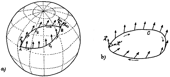
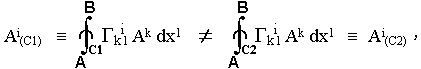
Fig.2.6. Parallel transmission in a curved space.
a ) In a
curved space (eg on a spherical surface), the result of the
parallel transfer of vector A from a given point A to point B depends on the path along which the
transfer takes place.
b ) This
non-integrability of the affine connection in the curved space
causes the vector transferred in parallel along the closed curve C
to differ from the original
vector after returning to the starting point.
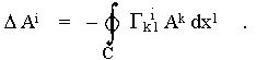
In the general case, however, Gk i l are functions of coordinates and parallel transmission according to equation (2.8) will depend on the path (Fig.2.6) - the connection will no longer be integrable :
where Ai (C1) are the components of the vector Ai transferred in parallel from point A to point B along
the curve C1, Ai (C2) is the result of the transfer
between the same points along the curve C2. In this case, if we perform a
parallel transfer with a given vector along a closed curve, we
return to the starting point generally with another vector
(Fig.2.6b). The size of this vector will be the same (the
invariance of the size of the vector in parallel transmission is
a basic requirement of the relationship between connection and
metric in Riemann space), its direction will change. Deviation of
this transferred vector from the original (relative to a unit of
area surrounded by a closed curve along which the transfer was
performed), is then a measure of
the nonintegrability of the connection and characterizes the difference
in geometric properties from Euclidean - it is a measure of the curvature of space.
A different measure of curvature of space is
based on the properties of the circle, respectively sphere. We construct the set of points having
the same distance r (measured along the shortest
path) from the fixed point O . In the two-dimensional case it
will be a "circle" and any difference in its length
from 2p r is a measure
of the curvature of the space (area); if the length of the
resulting curve is less than 2p r, the
curvature is positive (eg spherical surface), if this length is
greater than 2p r, the curvature is negative
("saddle" surfaces). Analogously, in three-dimensional
space geometric place the points having a distance r
from the center is formed by a closed surface, whose contents are
compared with the content of Euclidean balls 4p R2; similarly for higher
dimensions. Criterion based on a parallel transfer, however, is
more general since it does not requires metrics, connection are enough here.
The change of the vector in the parallel transfer of vector A along the closed curve C is
This curve integral generally cannot be converted to a area integral using the Stokes theorem, because the values of the component of vector Ai at the points of the respective area (inside the curve C) cannot be unambiguously determined - they depend on the path that the expansion of the vector field with a vector Ai at that point we come. However, if the curve C is sufficiently small (infinitesimal), this ambiguity does not apply in the transition to limit (the corresponding error is up to second order) and Stokes theorem gives (the variability of the vector field Ai with place is there only due to the connection, so ¶Ai/¶xl = - Gk i l Ak)
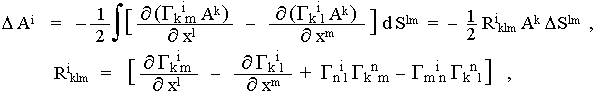 |
(2.18) |
where DSlm is the tensor of the area bounded by an infinitesimal closed curve C. A more detailed derivation can be found eg in [214], [166]. The tensor R i klm , which quantifies the difference between the geometric properties of a given space from the planar one (nonintegrability of the afine connection), is called the Riemann-Christoffel curvature tensor.
In flat space, the curvature tensor is zero everywhere, because you can choose a Cartesian coordinate system in which all Gk i l are zero everywhere, so that even Ri klm = 0; thanks to the tensor character Ri klm, this also applies to any other (perhaps curvilinear) coordinate system. Conversely, if Ri klm = 0 everywhere, the parallel transfer is unambiguous and path independent, so that a locally Cartesian coordinate system introduced at one point can be transferred in parallel and extended to all other points, ie construct a global Cartesian system Ţ space is planar. Equation
| R i klm = 0 | (2.19) |
is therefore a unequivocal criterion of whether the space described (using any coordinate system) by the given fields Gk i l , or gik, is flat or curved.
Here we mention some properties of the curvature tensor. From the definition of the curvature tensor contained in relation (2.18) it can be seen that the tensor Ri klm is antisymmetric in the indices l, m :
| R i klm = - R i kml . | (2.20) |
In addition, the tensor Ri klm is cyclically symmetric in its three covariant indices, ie.
| R i klm + R i mkl + R i lmk = 0 . | (2.21) |
Other algebraic relations (identities) hold for the covariant curvature tensor Riklm = gij Rj klm , obtained by reducing the index i:
| Riklm = - Rkilm = - Rikml , Riklm = Rlmik ; | (2.22) |
according to these
relations, those components of the curvature tensor which have i
= k or l = m are equal to zero.
A 4th order tensor in N-dimensional space
generally has a total of N4 components (in four-dimensional
space-time it is 256 components); however, due to the algebraic
identities (2.20) - (2.22), the number of algebraically
independent components of the curvature tensor is only N2
(N2 -1)/12 , ie only 20
independent components in four-dimensional space-time.
By narrowing the tensor Ri klm in the indices i and l (which according to identities (2.20) and (2.22) is the only narrowing giving a non-zero result) we get the so-called Ricci curvature tensor R ik
| R ik = def R m imk = g ml R milk , | (2.23) |
which is symmetrical. By further narrowing we get an invariant, which is called the scalar curvature R of the given space:
| R = def g ik R ik = g il g mk R milk . | (2.24) |
In addition to algebraic symmetries, the curvature tensor also satisfies important differential relations, the so-called Bianchi identities, between covariant derivatives of the curvature tensor :
| Riklm;j + Riklj;m + Rikmj;l = 0 . | (2.25a) |
Narrowing this equation in the indices i and l and by multiplying g jk we get, given the covariant constant of the metric tensor g jk ; n = 0, relation (Rj l - dj l R/2) ; j = 0, which can be written in the form
| Gik;k = 0 , where Gik =def Rik - 1/2 gik R . | (2.25b) |
This narrowed Bianchi identity, according to which the covariant four-divergence of the Einstein's curvature tensor G ik is identically equal to zero, plays a key role in the gravitational field equations, as we will see in §2.5.
The curvature tensor figures in all phenomena, in which the curvature of space (space-time) is applied. We will mention two such situations. In flat space, the second partial derivatives of the vectors according to the coordinates are commutative (Ai, k , l = Ai, l , k), as well as the covariant derivatives: Ai ; k ; l = Ai ; l ; k . In the general case, however, according to (2.13) applies
| (2.26) |
so the covariant
derivatives are generally non-commutative and the measure of this
non-commutativity is the curvature tensor Riklm .
In planar space, two lines passing
parallel through two points remain parallel at all times. In a
curved space, however, two geodesics (playing the role of lines
here), originally parallel in one place, gradually deviate from
each other due to the curvature of space. The equation of this deviation of geodesics (2.57) also shows the tensor of
curvature, as we will see in §2.6 "Deviation and gfocus of geodesics".
Generalization
of physical laws to curved spacetime
Because the actual
gravitational field is actually curved spacetime, the
extraordinary importance of the space-time curvature tensor in
gravity physics is obvious, where this curvature tensor expresses
the inhomogeneity of the
gravitational field. Already from Newton's theory of gravity
we know, the inhomogeneity of the gravitational
field is closely related to the excitation source of the
gravitational field. In §2.5 we will see that in Einstein's
theory of gravity the equations of gravitational field generation
put into context the curvature of space-time to the distribution
of excitation masses, ie they describe how matter curves space-time in its vicinity.
It is precisely such "corrections" on the connection as in (2.11) and in (2.15) that we have actually made in both examples at the beginning of the generalization of physical laws to curved spacetime. The equation of motion of a particle (2.5a) d2xi(l)/dl2 ş dui(l)/dl = 0 says, that along the world line of a free test particle, the four-velocity ui ş dxi/dl is constant. In general coordinates, the derivative dui/dl must be replaced by the absolute derivative (2.15), which gives equation (2.5b) :
| 0 = Dui /dl ş dui /dl + Gkil uk dxl/dl = d2ui /dl2 + Gkil (dxk/dl) (dxl/dl) . |
And in the equation of the law of conservation of energy and momentum Tik, k = 0, when transcribed into general (curvilinear) coordinates of normal partial four-divergence must be replaced by covariant four-divergence, which leads to equation (2.6), which according to the notation in (2.11) can be written in the form
| T ik ; k = 0 . | (2.6 ') |
We can therefore state the general rule of the relationship between the laws of non-gravitational and gravitational physics :
| Theorem 2.3 |
| The generalization of the physical laws valid in planar spacetime (ie the laws of special theory of relativity without gravity) to curved spacetime (presence of a gravitational field) consists in the fact that ordinary partial derivatives according to coordinates are replaced by covariant derivatives . |
In addition, the Minkowski tensor hik passes to the general metric tensor gik. Theorem (2.3) is sometimes abbreviated as the rule "replace commas with semicolons".
Let us now return to the physical meaning of the geodetic equation (2.5b). In the limit case of small velocities and weak fields (moreover, the field must be weak so that the particle does not gain high velocity in it), the general equations of motion of the particle in the gravitational field must pass to the corresponding non-relativistic equation (1.29b). To clarify the physical significance of geometric quantities of space-time, we compare equation (2.5b) with Newton's equation of motion for a situation where the gravitational field is still sufficiently weak. In this case, the tensor gik does not depend on the time coordinate x°, goa = 1 (a = 1,2,3) and there is a reference system in which the metric tensor can be decomposed into
g ik (x) = h ik + h ik (x) , | h ik | « 1 ,
where h ik are small deviations from the Minkowski metric. Such a system is approximately inertial with Cartesian coordinates around the test particle. Assuming that the motion of a particle in this frame of reference is not very fast (|v| «c, where v ş va = dxa/dt is the velocity of the particle), the proper time t will be approximately equal to the coordinate time t = x°/c, so in the geodetic equation we can put dxb/dt » dxb/dt = vb, dx°/dt » dx°/dt = c. If we limit ourselves to first-order members in h ik, will be the only nonzero components of the affine connection Gb oo = G°b o = - (1/2) ¶hoo/¶xb (b = 1,2,3). In this approximation, the spatial part of equation (2.5b) has the form
d2xa/dt2 - (c2/2) ¶hoo/¶xa = 0 .
If we compare it with Newton's equation of motion in the gravitational field (2.4) rewritten in the form
d2xa/dt2 + ¶ j /¶xa = 0 ,
we see that Newton's equation of motion is a special case of the general equation of motion of geodesy (2.5b), whereas the relationship between the usual gravitational potential j and the metric tensor is hoo = - 2 j/c2 , or
| g oo = - (1 + 2 j / c 2 ) . | (2.27) |
Again, this shows that the components of the metric tensor have the physical significance of the gravitational field potentials; Christoffel's affinity connection coefficients then express the gravitational forces acting.
If the "test particle" has zero rest mass and moves at the speed of light (eg photon), its motion in the local inertial system will be given by the equations d2xi/dl2 = 0, ds2 = c2 dt2 = hik dxi dxk = 0, where l is afinne parameter replacing the proper time t (which is not applicable here, because it is equal to zero). In general curved spacetime (in the gravitational field), the light propagation equation has the form
d2xi /dl2 + Gkil (dxi/dl) (dxk/dl) = 0 , ds2 = gik dxi dxk ,
where the second equation can also be written in the form (ds/dl)2 = gik(dxi/dl)(dxk/dl) = 0. The worldlines along which photons move freely are called light, isotropic, or zero geodesics (along them, the intrinsic time dt and the four-dimensional distance ds are equal to zero).
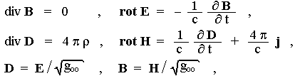
Gravitational electrodynamics and
optics
Using the rule contained in Theorem 2.3, it is easy to generalize
the specially relativistic equations of electrodynamics (derived
at the end of §1.6) so that they apply in curved spacetime, ie
in the gravitational field. The electromagnetic field intensity
tensor F ik = ¶ A k / ¶ x i
- ¶ A i / ¶ x k
will be defined here as F ik = A k;
i - A i; k , but it can be easily shown
that A k; i - A i; k = A k,
i - Ai, k . The relationship between the
four-potential A i and the electromagnetic field
tensor F ik therefore does not change. Similarly, the
first "pair" of Maxwell's equations retains its
(four-dimensional) shape :
| F ik, l + F li, k + F kl, i = F ik; l + F li; k + F kl; i = 0 . | (2.29) |
If we replace in the Lorentz equation of motion of charged test particles (mass m and charge q) in the electromagnetic field m.c.(dui/dt) = (q/c) Fik .uk the derivative dui/dt by the absolute derivative "Dui /ds", we get the equation of motion of a charged particle in an electromagnetic and gravitational field in the form
| mc . (dui /ds + Gkil uk ul) ş mc . Dui /ds = (q/c) Fik uk . | (2.30) |
The continuity equation j i , i = 0 will have a general form in curved spacetime
| j i ; i = 0 | (2.31) |
and a second portion of the Maxwell equations Fik , k = - (4p/c).j i in a gravitational field will be generalized to
| F ik ; k = - (4p/c). j i . | (2.32) |
Thanks to the antisymmetry of the tensor Fik, the continuity equation (2.31) follows again from this equation. The four-current density vector is defined in STR as j i = r .dx i /dt, where r = dQ/dV is the charge distribution density in space. After transformation into curvilinear coordinates, the element of volume dV passes into Ö(g) dV (where g is the determinant of the spatial metric tensor gab and dV = dx1 dx2 dx3 ) and the four-current in general equations (2.31) and (2.32) is given by
| j i = (r.c/Ögoo) . dxi/dxo . | (2.33) |
To clarify the effect of gravity on electromagnetic phenomena, it is interesting to decompose the equations (2.29) and (2.32) in three-dimensional form [166]. If we introduce quantities
Ea ş Foa , Da ş Ö(goo) F°a , Bab ş Fab , Hab ş Ö(goo) Fab ,
in them equations (2.29) and (2.32) will have the form after the separation of spatial and temporal components :
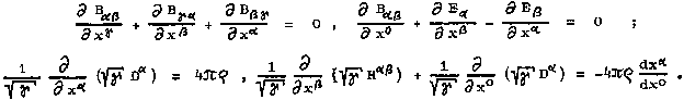 |
(2.29') (2.32') |
If the gravitational field is static, these equations can be rewritten in the usual (three-dimensional) vector symbolism :
 |
(2.29 '') (2.32 '') |
where vector H has components Ha = - (1/2) Ö(g) eabg H bg and vector B has components Ba = - (1/2 Ög) eabg Bbg . If we look at equations (2.29") and (2.32") from the point of view of non-gravitational physics - electrodynamics, these equations have the form of Maxwell's equations of the electromagnetic field not in vacuum, but in a material environment with dielectric constant and permeability
| e = m = 1 / Ö g oo . | (2.34) |
Thus we see that the gravitational field (curved
spacetime) has a similar effect on the electromagnetic field as
the electrically and magnetically "soft" substance - optical environment. The electromagnetic waves,
which are the wave solution of Maxwell's equations, will
therefore propagate unevenly and curvilinearly in the inhomogeneous
gravitational field, as can be seen, by the way, also from the
equation of zero geodesy (2.28) describing the motion of photons.
Due to the versatility of gravitational interaction, there is no dispersion; however, in contrast to conventional
optics of material environments, a frequency
shift is
manifested in the gravitational field (see
"Gravitational spectral shift" below) .
Therefore, we can expect interesting optical phenomena in strong inhomogeneous gravitational
fields - a kind of gravitational "fata morgana" -
similarly to optically inhomogeneous material environments. The
propagation of light in the gravitational field of a black hole
and the effect of a "gravitational lens" are mentioned
in §4.3, section "Gravitational lenses. Optics of black holes".
Space
and time in a gravitational field
Gravitational
time dilation
It still remains to clarifiy the relationship between the actual
time intervals and spatial distances in space events and their
coordinates xi in the general frame of
reference S . We start from the expression for an
invariant space-time interval
ds 2 = - c 2 d t 2 = g ik dx i dx k
and introduce an inertial frame of reference S~ such that it is currently at rest with respect to frame of reference S (with respect to its clock and measuring rods) at a given point. Then both the lengths of sufficiently short (infinitesimal) measuring rods and the time intervals will be the same in the system S and S~. In this locally inertial system S~ with the coordinatei x~ i is
ds2 = - c2 dt2 = hik dx~i dx~k = - (dx~°)2 + dx~a dx~a ,
where the relation between hik and the metric tensor gik is given by the transformation relation
| gik = hlm.(¶x~l/¶xi).(¶x~m/¶xk) = (¶x~a/¶xi).(¶x~a/¶xk) - (¶x~°/¶xi).(¶x~°/¶xk) . | (2.35) |
The inertial system S~ is locally at rest with respect to the general system S so that ¶x~ a/¶x° = 0 and the transformation relation dx~ i = (¶x~ i/¶xk) dxk has a separate form dx~° = (¶x~°/¶xk)dxk, dx~a = (¶x~a/¶xb)dxb. The relationship between the time coordinate x° and the proper time t can be easily determined by taking two events that occurred in short succession from the point of view of the reference system S at the same place. The interval between these events is then ds2 = - c2 dt2 = gik dxi dxk, and since dxa = 0, ds2 = - c2 dt2 = goo dxo 2 , ie
| d t = (1 / c). Ö (-g oo ) dx o . | (2.36) |
For a weak gravitational field using the relation (2.27) we get
| d t = (dx ° / c). Ö (1 + 2 j / c 2 ) » (1 + j / c 2 ) dt . | (2.36 ') |
Thus, the proper time with respect to the coordinate time (which corresponds to the zero gravitational potential) flows the slower, the higher the value of the gravitational potential j at a given location (the gravitational potential is negative) . The clock located in the gravitational field is delayed compared to the same clock located outside the field, resp. in a place with a weaker field.
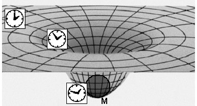 |
Gravitational
dilation of time. The clock located in the gravitational field is delayed compared to the same clock located outside the field (or in a place with a weaker field). |
In the vicinity of
material bodies (compared to distant
places) time flows more slowly *), there is a "slowing down of the flow of time through the
gravitational field" - a gravitational dilation of time. The
consequences of this phenomenon (such as
the gravitational redshift mentioned below) are crucial in the final stages of
gravitational collapse and the formation of black holes (see
§4.2,4.3).
*) If we took the anthropocentric
stand, we could say with a bit of exaggeration that "bodies
fall in the gravitational field because they are trying to reach
the place where they will age the slowest "..?..
This gravitational dilation of time is related to
non-inertial accelerated frames of reference, according to the
principle of equivalence. The value of the gravitational time
dilation at a given location in the gravitational field is the
same as the STR time dilation (1.72) caused by a velocity equal
to the escape velocity from that location.
Time dilation inside gravitational bodies
Ordinary gravitational bodies - planets, stars - have their mass
distributed in space of approximately spherical shape of radius R
with density r(r), where r is the distance from the center r =
0. For a spherically symmetric distribution, the Newtonian
gravitational force F (field
strength - force acting on a unit mass of the test particle) is given by the law of inverted squares (1.1). Outside the
body (r> R) is simply F(r) = GM / r2, inside (r <R) is F(r) = G. (0 ň r 4p r(r) r2 dr) /r2. Inside the body, therefore, gravitational force is smaller
in depth - is given only by the gravitational mass contained
between the given place r and the center r = 0. And in the
middle r = 0 the gravitational force is zero -
the gravity of the outer layers, acting in opposite directions,
is canceled (it was also discussed
in §1.2, passage "Gravitational
bodies"). However, it does not follow that the
gravitational dilation of time is also "cancel" here
and disappear !
The gravitational dilation of time does not depend on the
gravitational force, but on the gravitational potential
(2.36 '), which is j (r) = - r ň Ą F(r) dr. Although
there is no force in the center of a gravitational body, it has
the gravitational potential there in reverse the maximum size
- and therefore the gravitational dilation of time there will be
relatively the largest ! We can imagine it that
a certain velocity is also needed from the center to reach the
surface, which is then added to the escape velocity from the
surface.
From the point of view of GTR, the problem of
space-time geometry outside and inside gravitational bodies is
analyzed by the so-called internal Schwarzschild
solution (3.13b).
Spatial metric
The element dl of the spatial distance cannot generally be determined as the
interval between two infinitely close events occurring at the
same point in time by putting dx° = 0 in the expression for ds2,
because the relationship between the proper time t and the time coordinate x° is in
different places different. For get a relationship between the
actual length and the spatial coordinates xa (a = 1,2,3) we must therefore look
for elementary length measuring rod in resting locally inertial
system S~ dl~ 2 = a=1S3(dx~a)2 = dx~adx~a transform into a
general non-inertial system S . By describing the transformation
relationship (2.35) for the metric tensor we get
![]()
Since ¶x~ a/¶x° = 0, ¶x~°/¶xa = - goa/Ö-goo, for the proper length of the infinitely short measuring rod then we get the relation *)
| (2.37) |
and for the interval of
the proper time we get dt2
= - (1/c2) goo dx°2
in accordance with (2.36). The expression in parentheses (2.37)
therefore indicates the metric of
three-dimensional space in the presence of gravity (or in a
non-inertial frame of reference), ie the three-dimensional metric
gab "induced" by the space-time
metric gik .
*) Another derivation of the relation
(2.37) by light signal propagation analysis ("radar"
distance) is given in [162], [135], [166].
By separating the spatial terms in the identity gik gik = 0, the relationships between the metric of space and spacetime can be derived:
| g ab = - g ab ; g oo g = - g , | (2.38) |
where g is the
determinant composed of gik and g
is the determinant of the components ga
b .
In order for a
reference system corresponding to the metric tensor gik to be physically feasible (using real
bodies), the three-dimensional metric form (2.37) must be positive definite and according to (2.36) goo <0. These conditions, expressed using
determinants and subdeterminants of the metric tensor, are called Hilbert conditions [162] :
| det | | | |
g oo g 10 |
g 01 g 11 |
| | |
< 0 , | | | g oo | g 01 | g 02 | | | > 0 , | g < 0 . | (2.39) |
| det | | g 10 | g 11 | g 12 | | | |||||||||
| | | g 20 | g 21 | g 22 | | |
Static and stationary
gravitational field
If there is a reference system in which the components of metric
tensor gik do not depend on the time coordinate x°,
the respective gravitational field is
called stationary. In addition, if there is a frame of
reference in a stationary field in which all "mixed"
components of the metric tensor goa are equal to zero, it is a static gravitational field in which both
directions of time flow are equivalent. It follows from Newton's
(as well as general Einstein's) law of gravitation that static
gravitational fields are excited by the static distribution of
matter; in §3.4 it will be shown that the gravitational field in
vacuum of spherically symmetrical body it is a static even when
this body radially pulses (expands or collapses). In practice, a
stationary gravitational field can only be excited by a compact
isolated body, because in a system of several free bodies their
gravitational interactions will cause mutual movements and the
resulting gravitational field will be variable. An example of a
stationary field is a gravitational field around an axially
symmetric body evenly rotating around its axis; however,
this field is not static, because both directions of time flow
are not equivalent here (when the direction of time is reversed,
the sign of the angular velocity of rotation of the body
changes). Indeed, according to Einstein's equations, the rotation
of the source body leaves "traces" in the form of
nonzero components goa of metric tensor on the metric of the
surrounding spacetime, see §2.5. Some interesting effects taking
place in the gravitational field of rotating objects (especially in
the vicinity of rotating black holes) will be discussed in §4.4.
Gravitational spectral shift
We will mention another important consequence of the gravitational dilation of time, the relationship between the
interval of proper and coordinate time (2.36) - the gravitational spectral shift, which we have already mentioned
above. According to the relation (2.36) in two places with
different gravitational potential, to the same coordinate time
interval will correspond the different intervals of the proper
(own) time. Let stationary gravitational field at point P1 is a
light source which transmits two light impulses discrete interval Dt(P1) of its own time; the coordinate
time interval between these events will then be Dt(P1) = (1/c)Dx°(P1) = (1/c)Ö(-goo(P1)).Dt(P1). These
light signals will propagate through space and be captured by the
observer at point P2 . Because in a stationary gravitational
field component metric tensor do not depend on the time
coordinate, the interval of coordinate time Dt(P2) between
the moment of receipt of both pulses the same as at the sending
point, i.e. Dt(P2) = Dt(P ). Because
Dt(P2) = Ö(-goo(P2)).Dt(P2), will be
| (2.40) |
Similarly, if a periodic radiation-emitting process (eg excited light-emitting atoms) takes place in a stationary gravitational field at point P1, then the number of oscillations per unit coordinate time will be the same at all points of the propagating radiation trajectory and the ratio between periods T(P1) and T(P2) radiation at P1 and P2 will again be given by (2.40). The frequency ratio will therefore be
| (2.41) |
In a weak gravitational field, goo(P) » -(1 + 2j(P)/c2), so
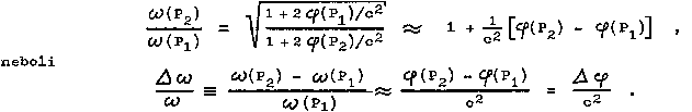 |
(2.41 ') |
If light comes from a
place with a higher gravitational potential to a place with a
lower potential, its frequency decreases - it is a gravitational
redshift. Conversely, when radiation propagates
from places with a lower gravitational potential to places with a
stronger gravitational field, a blue
shift occurs -
the frequency of light increases.
Thus, the gravitational frequency shift
results from the geometric interpretation of the gravitational
field in the general theory of relativity. However, the same
conclusion, including the relation (2.41 '), can be reached by
more elementary procedures. The first of these is the kinematic interpretation using principle
of equivalence:
a situation where the light source and the receiver (observer)
are located in places with different gravitational potential, we
replace the equivalent state in which the light source and the
observer are located in different places of a uniformly accelerated reference system (for example, in the rocket
cabin as in Fig.2.3b). From the time moment t = 0 of sending light from
point P1 to the moment Dt = DL/c of its registration by a receiver
located at a distance DL in the direction of
acceleration, this receiver obtains the relative velocity v = a. DL/c. Therefore, due to the Doppler effect, the wavelength of the received light
will appear different from the wavelength l of the radiation
emanating from the source, this deviation expressed by the
frequency w will be in the first order
Dw / w » v / c = a. D l / c 2 .
Returning now to the
initial situation with the gravitational field, then the quantity
a.Dl means the difference of the
gravitational potentials Dj between the source and the
receiver, so when overcoming the difference of the gravitational
field potential Dj = a. Dl, the
wavelength of light changes by Dj/c2
in accordance with the formula (2.41').
Similarly, the gravitational
dilation of time
can be determined according to the principle of equivalence in a
uniformly accelerated frame of reference as STR dilatation of
time when we substitute the above-mentioned relative velocity
into the relation (1.70) in §1.6 v = a. Dl/c :
Dt ' = Dt / Ö (1 - a2 Dl 2 / c4 ) .
The change in frequency Dw/w resulting from this time
dilatation will be in the first order
approximation ~ a. Dl/c2, which, expressed by the potential difference, again
gives Dj c2.
The gravitational frequency shift can also
be easily derived as a consequence of the law
of conservation of energy during the motion of photons in the classical gravitational
field. The light of wavelength l and
frequency w we consider
as a stream of photons with energy E = h.w = h l and mass m = E/c2. When the potential difference Dj in the gravitational field is overcome,
the energy of the photons changes by DE = Dj .m = Dj
.E/c2,
so that the relative change in wavelength is again Dj/c2 .
Pound-Rebka experiment
Although the gravitational frequency shift is completely
insignificant in terrestrial conditions and does not manifest in
practical life, the gravitational red shift was succeeded experimentally demonstrated and measured even in the Earth's
gravitational field. In 1960, R.V.Pound and G.A.Rebka [208] for
this used the Mössbauer effect *) of resonant nuclear
absorption of g- radiation with an energy of 14.4
keV of the excited level of a 57Fe iron nuclei. Source - b + g radioisotope 57Co with mechanical shift (periodical shift by electro-mechanical movement of the
loudspeaker diaphragm) and receiver (absorber 57Fe with spectrometric radiation detector g) were located in the water tower at
Harvard with a height difference of only 22.5 meters. Two
measurements were made while exchanging the positions of the
transmitter and receiver (ie, both red and blue shifts
were measured) to exclude non-gravitational shifts of the
spectral line. The measured values of the relative frequency
shift of about 2.5.10-15 agreed with the formula (2.41')
originally with an accuracy of about 10%, in the improved variant
of Pound and Snyder the agreement improved to 1% [209].
*) The Mössbauer effect is described in
more detail in the book "Nuclear Physics and Physics of
Ionizing Radiation", §1.6 "Ionizing
Radiation", part "Interaction
of gamma radiation",
passage "Resonant nuclear
absorption - Mössbauer effect".
Gravity
Probe A
With even greater accuracy, the gravitational frequency shift was
measured in 1976 on a strongly eccentric elliptical orbit (so
that the probe passed the largest possible difference in
gravitational potential of Earth) of the disposable satellite Gravity
Probe A (maximum height of the
suborbital orbit, ie a turning point of 10,000 km above Earth,
flight time 55min, end of runway in the Atlantic). An accurate clock equipped with a hydrogen MASER was
installed on the satellite, the same MASER was placed in a
control center on the Earth's surface. By comparing the
registered data, the gravitational redshift was measured, which
agreed with the GTR with a relative accuracy of 2.10 -4 .
Astronomical measurements
of the gravitational redshift
In addition, there are astronomical
verifications of the gravitational redshift. The light emitted
by atoms from the surface of the Sun arrives on Earth according
to the relation (2.41') with a redshift of Dw/w @ 2.10-6, which is a few percent of the
width of the Fraunhofer lines. This effect is well measurable by
spectroscopic methods, but in addition to the Doppler shift
correction by due to the relative radial motion of the
Earth and the Sun, the flow of hot gases on the surface of the
Sun is significantly manifested here. Hot gases rise, cool at the
surface and fall back. The value of the redshift corresponding to
the relativistic formula (2.41') is measured directly only from
the areas at the edge of the solar "disk", where the
radial streams of glowing hot gases are observed perpendicularly.
In contrast, the red shift of radiation from a central region of
the solar disc is very small and the spectral lines are Doppler
shift due to the rising their hot and descending cooler streams
of gas glowing extended and asymmetrical, with the center
position is shifted to higher frequencies. Using a detailed
analysis of the peak shape of these spectra [216], it was
possible to correct the effect of the Doppler effect radial
streams of hot gases on the surface of the Sun and show that the
gravitational redshift is approximately the same in all places of
the solar disk and coincides well with the relation (2.41') (accuracy about 5%).
A significantly higher redshift can be
expected for massive compact stars such as white dwarfs (see
§4.2), on the surface of which the gravitational potential is
one to two orders of magnitude stronger. For measurement and
comparison with the relativistic prediction, only bright white
dwarfs are suitable, which are part of binary stars, in order to
determine their mass. However, the radius of a white
dwarf of known mass cannot be determined directly, but only on
the basis of the theory of the structure of white dwarfs;
therefore, the measurement of the red displacements of white
dwarfs can be considered as a test of the theory of their
internal structure rather, than as a verification of the
relativistic relation for the gravitational red displacement.
E.g. for Sirius B, which has a mass approximately the same as the
Sun, the theoretical radius is about 10-2 solar radius and the redshift is
thus 2.10-4; however, interferes with accurate
measurement of strong light transilumination from nearby Sirius
A. Somewhat favorable situation is with the binary 40 Eridani a
greater distance of the two components, wherein the white dwarf B
measurement leads to an agreement about 20% of a theoretical
value of red shift [207].
More
complex effects of frequency shifts can be expected with relic
radiation, which on its long journey through vast cosmic
spaces passes through areas with a large accumulation of matter
in galaxy clusters and, conversely, large areas of
"emptiness". These fluctuations in
gravitational potential and space-time metrics may slightly modulate
the anisotropy of relic microwave radiation (see §5.4, section "Microwave relic radiation", section "Influence
of gravitational fluctuations in space metrics on relic radiation
- Sachs-Wolf effect") .
| Gravity, black holes and space-time physics : | ||
| Gravity in physics | General theory of relativity | Geometry and topology |
| Black holes | Relativistic cosmology | Unitary field theory |
| Anthropic principle or cosmic God | ||
| Nuclear physics and physics of ionizing radiation | ||
| AstroNuclPhysics ® Nuclear Physics - Astrophysics - Cosmology - Philosophy | ||