 |
|
| Derivative of the function f(x) | Integration of the function f'(x) |
| AstroNuclPhysics ® Nuclear Physics - Astrophysics - Cosmology - Philosophy | Gravity, black holes and physics |
Chapter 1
GRAVITATION AND ITS PLACE IN PHYSICS
1.1. Development of knowledge about nature,
universe, gravity
1.2. Newton's law of gravitation
1.3. Mechanical LeSage hypothesis of the
nature of gravity;
1.4. Analogy between gravity and
electrostatics
1.5. Electricity and magnetism. Maxwell's equations.
Electromagnetic waves.
1.6. Four-dimensional spacetime and
special theory of relativity
1.5. Electricity and magnetism. Maxwell's equations. Electromagnetic waves.
The most important force that determines all
internal structure and behavior of natural objects, from
subnuclear, atomic, and molecular scales, to the macroscopic
dimensions of surrounding nature (including ourselves) and the
scales of the Earth and other planets, is electromagnetic
interaction. Carriers of electric forces are
the basic building blocks of atoms - electrons
carrying a negative elementary electric charge
and protons carrying a positive charge (positive and negative signs evolved by convention). The electric forces between protons and electrons, in
co-production with quantum laws, determine the structure
of atoms, and thus the chemical and
physical properties of substances (... "Interaction
of atoms" ...).
Each electric charge (charged body)
excites an electric field around it according to
Coulomb's law (1.20b) with an intensity proportional to
the magnitude of the charge and inversely proportional to the
square of the distance; if the charge does not move (in the given reference system),
it is an electrostatic field. The electric field exerts force
effects on every other charged body that enters this space.
If the charge moves (it is an electric
current), in addition to the electric
field, it also excites a magnetic field
according to Biot-Savart-Laplace's law (1.33a). The
magnetic field shows force effects on each electrically charged
body that moves perpendicular to the direction
of the magnetic field vector (Lorentz force). The
combination of both fields represents an electromagnetic
field. When electric charges move at a variable
speed (with acceleration or
deceleration), they create a time-varying
electromagnetic field around them, which leads to the formation
of electromagnetic waves that detach from their
source and carry some of its energy into space. According to
Faraday's law, electromagnetic induction of an
electric field arises when motion or time changes in a magnetic
field; and temporal changes in the electric field in turn cause a
magnetic field. This field is governed by Maxwell's
equations of the electromagnetic field, which were
created by combining and generalizing all the laws of electricity
and magnetism. The combined science of electricity and magnetism,
including the dynamics of charge motions and the time variability
of fields, is called electrodynamics. This will
be the main content of the existing §1.5.
In the previous §1.4 we saw that
the analogy between Newton's gravistatics and Coulomb's
electrostatics is very tight. However, the electrostatic field is
a special case of the general electromagnetic field that prevails in the
vicinity of moving electric charges. It is therefore useful to
note the properties of the electromagnetic field and to try to
find possible analogies with the general "gravidynamic"
field around moving bodies. Electrodynamics is the most perfect and
successful theory of classical physics, which retains its full
validity even in modern relativistic physics. It can be said that
electrodynamics is one of the cornerstones
of all physics and has played a key role in shaping the
special and general theories of relativity, as well as quantum
physics.
Note: The historical
development of knowledge about electricity and magnetism is
briefly outlined in §1.1 in the passage "Electrodynamics,
atomic physics, theory of relativity, quantum physics". The relativistic view of the relationship
between electric and magnetic fields is briefly discussed below
in the section "Relativistic Electromagnetism".
Linearity of electromagnetism :
Electric and magnetic action in vacuum is linear in sources (electric charges of different
sizes) and in the values of fields excited directly or
by induction. The principle of superposition
applies here exactly. The values of electric and magnetic field
intensities from different sources are simply added up
(vectorially). This is no longer entirely true in the material
environment, where the effects of interactions of
electric and magnetic fields with the configurations of atoms
in materials are applied. Below we will see that this can occur
when an electric field is excited by charges in inhomogeneous
dielectrics, at their interfaces, and especially when a magnetic
field is excited in ferromagnetic substances, where the
saturation state also manifests itself.
In quantum field theory, higher-order effects occur when
photons interact through fermion loops. We leave aside here the
hypothesis of nonlinearity of electrodynamics at superstrong
field intensities ("Nonlinear electrodynamics")...
Physical units in
electricity and magnetism
During the long-term development of physics and natural science,
not only were new knowledge constantly acquired, but also various
physical quantities and units for their quantification were
introduced. Particularly dynamic development and abundance of
various units took place in the field of electricity and
magnetism during the late 18th to the first half of the 20th
century.
Systematic work on the creation of a unified and
rational system of physical units began in 1862 on the
initiative of the British Association for the Advancement of
Science. Thus, the "absolute" CGS
system was created based on three basic units: Centimeter,
Gram, Second. The International
Conference on Weights and Measures was established and etalons
for the meter and kilogram were implemented. However, there were
many different electrical and magnetic units, often based on
secondary empirical knowledge (e.g. the Ampere unit based on the
decomposition of silver by electric current during electrolysis,
or the Ohm using the electrical resistance of a mercury column).
From the point of view of the nature and connection of phenomena,
the CGSE system proposed by C.F. Gauss is often
used in fundamental (theoretical) physics, which assumes the
coefficients e0 and m0 to be equal to 1 - it includes them in the quantities
of electric E and magnetic B
field intensities. This leads to concise and concise notations of
equations between electromagnetic quantities. We will mostly use
them in theoretical analyses. However, we will also present
important resulting formulas and practical applications in SI
units.
The international system of units SI
developed mainly in the first half of the 20th century. The three
basic mechanical units meter, kilogram and second were
supplemented by the electrical unit ampere in 1950 -
thus the MKSA system was created. In 1960, the
International Conference on Weights and Measures named the system
based on the meter, kilogram, second, ampere, kelvin and candela
"Systeme international d'unités"
(International System of Units) with the abbreviation SI.
For technical applications, the SI system is now the
most practical and almost exclusively used, because its units are
mostly close in size to the dimensions and intensities in common
nature; and also because all current measuring instruments are
calibrated in these units.
Note: Incorrect or illogical definition
of the basic units of electromagnetism !
The historical development of the knowledge of basic physical
laws sometimes took quite convoluted paths. Along with this,
definitions of physical quantities and their units
were also formed, which were indebted to the ideas of the time.
The introduction of electric current as a basic
quantity and its SI unit Ampere (using the "magnetic force
action of two infinite parallel conductors...") was
unfortunate. Physically, the primary thing is
the electric charge, from which the electric current
should be derived as the amount of charge passed per unit of time
(Coulomb/second). Or in magnetism, the terminological
illogicality of the names "magnetic field intensity"
and "magnetic induction" - it should be the
other way around! - (for an electric field, it is fine). It is
briefly discussed below in the passage "Intensity<->Induction
in electromagnetism". This
unfortunate "crossing" of the names "intensity-induction"
arose during the historical development of the science of
electricity and magnetism, when magnetism was mistakenly
explained by fluid theory, analogous to electrostatics.
And unfortunately, it has remained so in the current SI system
...
Integral and differential
formulations of physical equations
Electrodynamics is a branch of physics where derivatives and
integrals of vector fields are used most in mathematical
formulas, often unified into the formalism of differential
operators. Fellow physicists are certainly well acquainted with
these techniques, but for those interested in other fields, I
would like to try to write a few notes here about their essence
and benefits. Physical fields are expressed by the values f
of forces-intensity and energies-potentials at different
locations in space. They are therefore functions of location
- of spatial coordinates x,y,z and time t - f(x,y,z,t).
We will first show this on functions of one variable f(x) and
their graphical representation.
To analyze natural processes in various situations, it
is often necessary to find out how quickly (how sharply,
with what gradient) one parameter changes in relation to another
parameter. This is quantified by the mathematical operation of
the derivative of one parameter with respect
to another parameter - it is written d f(x)/dx| x=x0 at the point x0, it is also denoted f
'(x). It is the steepness of the change in the value of this
function with respect to an infinitesimal change in its
independent variable. In mechanics, the derivative of position
with respect to time expresses the speed of movement of
a body. For a function of one variable f(x), the derivative
determines the slope of the tangent to the curve of its
graph at a given point x0. For functions of several variables f(x,y,z,t), partial
derivatives ¶f/¶x, ¶f/¶z, ¶f/¶z, ¶f/¶t are introduced - partial gradients in the direction of
individual coordinate directions x,y,z and time t. Here,
only the variable with respect to which the derivative is made is
taken as a variable, while the other variables are considered
constant.
|
|
| Derivative of the function f(x) | Integration of the function f'(x) |
We often also need to add-sum the
local instantaneous values of a certain quantity into the
resulting accumulated value, which can determine the
functional behavior of other quantities. If these are constant
values, it is a simple arithmetic operation of "+"
addition. However, with variable values of the function f(x),
this addition must be performed gradually, locally as integration.
It is written nf(x) dx. The integral sign n is a
vertically extended band "S", an abbreviation for summation.
The integrated range x1÷x2 is divided into infinitesimal sections dx and the
elementary products f(x1+n.dx).dx are gradually added until x2 is reached. The
integral of the function f(x) gives the area under its curve
between the values x1 and x2.
In a two-dimensional generalization, for functions of
two variables f(x,y), integration is done using infinitesimal
parallelograms and the area integrals Snnf(x,y) dS of either scalar quantities (such as mass or charge using their areal density) or the flux of a vector field over some given area S
are computed. Next, curve integrals are computed
along some parameterized curve in the 2-D plane. Area integrals
of vector functions can be converted to volume integrals using
Gauss's divergence formula, or to line integrals using Stokes's
rotation formula - see the figure below.
Differentiation and integration
of functions
Above, we outlined the derivative of the function f(x) at a
specific point x0 and its integral in a certain range x1-x2. The result is a
certain local number. However, for a more complete
analysis of the behavior of functions, it may be important to
perform the differentiation and integration operations at all
locations of the function f(x) - for all values of the
variable x (in a given domain of
definition). The result of this process is
then a new function f '(x) or F(x), which shows the
differential or cumulative trend of the original function f(x).
By differentiating the function f(x), the function f
'(x) is created, which quantifies the variability of the
original function f(x) at each location when the independent
variable x changes. In places where the function f(x) is
increasing, the derived function f '(x) is positive and its value
is proportional to the steepness of the growth, in decreasing
regions of f(x) the derivative goes to negative values. Where
f(x) is constant, or has local maxima or minima, the derivative f
'(x) is zero.
The integral nf(x) dx = F(x) is called an indefinite integral,
because it has no specified limits for the independent variable x,
it is integrated continuously over the entire domain of the
function f(x). If the function f(x) is nonnegative, its integral
F(x) is a monotonically increasing function. If the function f(x)
also goes to negative values, negative values may also prevail
even in the integrated function F(x).
 |
|
| Differentiating the function f(x) gives the function f '(x) | Integrating the function f(x) gives the function F(x) |
Differentiating and integrating functions are mutually opposite processes - from the derived function f ´(x) we can obtain the original function f(x) by integrating, using the initial condition. Conversely, from the function F(x) we can obtain the original function f(x) by differentiating. The function F(x) is sometimes called the "primitive function" of the function f(x).
Differential operators
Derivatives of vector field functions (here electric and magnetic
field intensities) are combined-unified into the
formalism of the so-called differential operators
for better clarity :
Nabla N: The basic differential operator here is
"nabla N": NF = ¶F/¶x + ¶F/¶y + ¶F/¶z . Other
derivative combinations are then derived from the operator N
:
Gradient: grad F = NF = [¶F/¶x, ¶F/¶y, ¶F/¶z] quantifies the
steepness of changes in the scalar field F at different
locations. In electrodynamics, this is the gradient of the
potential f.
Divergence of the vector function F:
div F = N . F
= ¶Fx/¶x + ¶Fy/¶y + ¶Fz/¶z. It quantifies
the local flow - divergence, convergence - of the vector field F.
In electrostatics it expresses the way in which the distribution
of electric charges creates the electric field E
- (1.32b).
Laplace operator: D f = div grad f = N2 f
= ¶2f/¶x2 + ¶2f/¶y2 + ¶2f/¶z2. It
quantifies the dynamics of the change of the field F
in space. In the 4-dimensional formulation x,y,z, c.t of the
special theory of relativity, the d'Alembert differential
operator š f
= ¶2f/¶x2 + ¶2f/¶y2 + ¶2f/¶z2 -
(1/c2)¶2f/¶t2 is
used.
Rotation or curl is the vector
product of the operator nabla N and the investigated vector function F:
rot F = N × F
= [(¶Fz/¶y - ¶Fy/¶z)+(¶Fx/¶z - ¶Fz/¶x) + (¶Fy/¶x - ¶Fz/¶z)]. It quantifies the
local rotation - circulation - turning - of the vector
field, changes in the direction of the vector F in the
vector field. It is expressed by the differences of the partial
derivatives Fx,y,z between the coordinates x,y,z. It is very well suited
for modeling the magnetic field B, which has a circular-spiral
shape around the exciting moving charges or fluxes -
(1.33)-(1.37).
The connections between the differential
relations and the integral dependencies of physical
quantities, here the field intensities and potentials, are
important here. For the differential operators "div"
and "rot" two important integral
equations hold :
--»
The Gauss-Ostrogradsky divergence formula shows
that the area integral of the vector field F(x,y,z)
over a closed surface S is equal to the volume integral of
the divergence of the field div F over the
volume V inside this closed surface. This means that the
flux of the vector field F over a closed surface
S is equal to the volume integral of the divergence of the
field div F, i.e., the local increments and
decrements of the field F, in the inner region
enclosed by the surface S.
--»
The Stokes integral rotation formula shows that
the flux of the vector rot F through the surface
S in space is equal to the curve integral of the
circulation of the vector F along the
curve C that bounds this surface. We can imagine this as
the local rotations of the vector field F
on the surface S are added to the resulting circulation of
the vector field F along the total curve C
bounding the surface S. For the magnetic intensity vector B
see formula (1.34.b), (1.37.b).
 |
|
| Gauss-Ostrogradsky divergence formula | Stokes integral rotation formula |
Electric charge
The name "electric charge" is used in
electrodynamics in two meanings :
1. A body or particle that exhibits a force of electrical
action. We also say that it is a carrier of electric charge.
They are primarily electrons and protons, and then ions and
bodies that have a mutual excess of electrons or protons.
There are also other charged particles in
the microworld - muons, pions, hyperons (§1.5 "Elementary
particles and accelerators", part "Elementary
particles and their properties"),
which, however, are very unstable, do not occur in our nature and
have no significance for the science of electricity importance.
2. A physical quantity that quantizes the size - the
measure of electric charge. The basic unit of charge is 1
Coulomb. In atomic and nuclear physics, the electron charge 1 e =
1.602x10⁻¹⁹ Coulomb is also
often used as a unit.
In field theory, the distribution of
electric charges is expressed by the charge
density r(x, y, z, t), which is generally a
function of place and time, so that the total charge contained in
the spatial region V is Q = V
òòò
r dV.
In an electromagnetic field acts on a test
particle with a charge q moving at a velocity v the
total force (Lorentz force)
| F =
q . E + q . [ v
x
B ] , electric force magnetic force |
(1.30) |
where E is the intensity of the electric field and B is the intensity of the magnetic field (for historical reasons called magnetic induction), "x" means the vector product. Below, we will first discuss the origin and properties of electric and magnetic fields separately, and then their mutual connections and dynamic behavior in the electromagnetic field.
Movement of electric
charges - electric current
In the science of electricity, the movement of electric charges
is generally called an electric current. Of
particular importance is the orderly movement of
charges, especially in conductors. In a narrower sense, the ordered
movement of electric charge carriers is therefore called an
electric current. It is quantified by the electric current I,
which is the electric charge q passing through the cross-section
of the conductor per unit of time: I = dq/dt. The unit in the SI
system is 1 Ampere, which is the charge of one Coulomb passed in
1 second (the awkward technical definition
of 1A using the "force action of two infinite parallel
conductors" is not important to us).
According to the type and movement of the
charge carriers, the electric current is divided into two basic
groups :
-> Conductive - drive current is an
ordered flow of free charge carriers in a material environment
under the action of an electric field. Above all, it is the
movement of free electrons in metal conductors, the movement of
ions in electrolytes or in gases during electric discharges.
Particles carrying an electric charge collide with atoms of a
substance as they move through the medium, transferring part of
their kinetic energy to them and causing them to oscillate. This
results in losses of electric current energy and heating of the
medium. A conductive medium offers a certain resistance to the
electric current (minimization or almost nullification of
resistance is discussed in §..., passage
"superconductivity").
-> Convective - flowing electric current
caused by the mechanical movement of charge carriers in
the environment, without the instantaneous effect of an electric
field (the charge carriers are either
carried by the flowing material medium, or move by inertia in a
vacuum). An important example of convection
current is the movement of charged particles in accelerators. In
a convection current, there are no collisions of charged
particles with particles of the environment, so there are no
thermal effects, but only electric and magnetic ones.
In terms of the time course and direction
of charge flow, we encounter two types of electric current :
-> Direct current, in which electric
charges do not change the direction of their flow over
time. The magnitude of the current can be either constant
over time (during the monitoring period of
the function), or variable -
increasing, decreasing, pulsating (while maintaining the same
direction). The source of direct current is, for example,
electrochemical galvanic cells and accumulators, thermocouples,
photovoltaic cells. Common electronic sources are rectifiers
that obtain direct current from alternating current.
-> Alternating current, which periodically
changes the direction of its flow over time. The periodic
waveform can be different, for example, rectangular (simple alternation of "+" and "-"), sawtooth, but the most common
is sinusoidal - harmonic: I(t) = Imax
. sin(w.t + j), where Imax is the amplitude, w is the angular frequency related to the frequency f
by the relation w = 2p.f a j (0÷360°) is the phase shift of the beginning of the
time coordinate t (or the phase
shift between voltage and current). The frequency
f indicates the number of oscillations per unit of time;
the unit 1 Hz means one oscillation per 1 second (the name is after one of the pioneers of
electromagnetism H.Hertz). Opinions on what
is low-frequency or high-frequency differ, depending on the field
in which alternating current is used. In everyday life and in
electroacoustics, 20 kHz is usually taken as the limit. In radio
engineering, this limit is usually moved up, to the MHz range...
We basically have two types of alternating current sources :
--» Alternators are rotary power
electro-mechanical sources of alternating current for energy
needs. The source of mechanical energy is a rotating turbine
- steam in thermal and nuclear power plants, or water in
hydroelectric power plants (or a propeller
in a wind source). The turbine drives the
magnetized rotor of the alternator, which creates a rotating
magnetic field. An alternating voltage with a
frequency given by revolutions/s is then induced in the stator
coils. Alternators in power plants have three coils
wound in their stator, angularly offset by 120°, thus creating a
3-phase current. In the globally interconnected
electrical network, all alternators operate synchronously with a
frequency of 50 Hz, in the USA with a frequency of 60 Hz.
Small and much simpler 1-phase alternators
with a voltage of about 14V are used in cars with an internal
combustion engine, that drives them and they charge the battery
and power the ignition, headlights and other electrical
equipment..
--» Oscillators are electronic circuits in
which periodic oscillations of electrical voltage and
current occur with a frequency dependent on the parameters of the
components (capacitors, coils, resistors,
transistors) and can often be tuned. Mostly
harmonic sinusoidal oscillations are created (exceptionally rectangular or sawtooth in multivibrators) for use in radio engineering or
instrumentation (for more details, see
"Transmission
and reception of electromagnetic radio waves" below).
Electrical components and
circuits in electronics
In the practical use of electricity, electric current and
voltage, electrical components (elements) with various required
properties are used. From the point of view of supplying or
consuming electrical energy, we can divide these components into
two categories :
-> Active -
sources, which supply electrical
energy to the circuit. In heavy-current power engineering, these
are electro-mechanical generators (alternators,
dynamos), which use rotating turbines or propellers to convert
the mechanical energy of steam, water or wind into electrical
energy. Then there are photovoltaic cells and galvanic cells. The
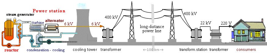
picture on the left shows a schematic representation of the
production of electrical energy in a power plant (nuclear here),
the transformation of voltage from 6 kV to 220-400 kV, in the
middle is the long-distance line to the consumption area. For
long-distance energy transmission, it is advantageous to
transform to high voltage, where a relatively small current
is sufficient, which minimizes ohmic losses in the line and also
thinner wires are sufficient (mostly Al-Fe
ropes with a cross-section of about 300mm2 are used). However, if the
voltage is too high, about >500kV, losses increase again due
to air ionization and small corona discharges. The picture on the
right shows a schematic representation of the transformation to
22 kV in a transformer station and finally to 220 V for powering
common electrical appliances at consumers :
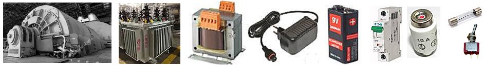
Production
and distribution of electrical energy
In addition to these basic primary
sources, there are secondary electronic sources,
which use this primarily created electricity to power the
resulting electrical circuits in household appliances, industrial
machines and laboratory instruments - transformers, rectifiers,
converters :
| Power supply of electrical circuits | |||||||||
 |
|||||||||
| Alternator in a power plant Power transformer Instrument transformer Small transformer Galvanic battery Fuses, circuit breakers and switches | |||||||||
-> Passive
components, which take electrical energy and convert it into
other types of energy (thermal, light, mechanical, sound,
electromagnetic...). We will mention a few of the most common
electronic components :
=» Resistors,
whose task is to provide a certain increased resistance to the
electric current, which reduces the electric current and
creates a certain voltage drop across the resistor. When
a stronger current (e.g. several Amps) passes through the
resistor, considerable heat is generated, so resistors can also
be used as heating elements. The unit of electrical
resistance is 1 Ohm [?]: A resistor has a resistance of 1? when a
current of 1 A flows through it at a voltage of 1 V. Resistors
are made of conductive materials with increased resistivity, such
as alloys of iron, nickel and chromium, or copper and nickel, for
higher resistances graphite. Either in the form of metal
resistance wires, or thin layers of graphite or metallic or metal
oxide layers, deposited on insulating (usually
ceramic) carriers with milled grooves to increase the
length of the layer and thus increase the resistance. A resistor
with a controllable adjustable resistance using a third
electrode, mechanically moved along the resistive layer, is
called a rheostat or potentiometer (the
name comes from the fact that it is a resistive voltage divider
previously used in devices for measuring electrical potential,
voltage).
=» Capacitors sometimes also
called condensers. The basic design of a
capacitor consists of two conductive plates (electrodes),
separated from each other by an insulating layer of dielectric.
When electric charges of opposite polarity are applied to each of
the plates and attract each other, the insulating dielectric
between them does not allow the charge carriers to come into
contact. The plates remain charged even after the electrical
source is disconnected. The basic property of a capacitor is to
accumulate an electric charge Q. This ability is
quantified, in relation to the electric potential - voltage U,
by a quantity called capacitance C = DQ/DU. In general, every
conductive body has an electric capacitance. The unit of
capacitance in the SI system is 1 Farad: A body has a
capacitance of 1 Farad if the supply of 1 Coulomb of charge
increases its voltage by 1 Volt. 1 Farad is a very large unit,
therefore its decimal fractions are used: microfarad 1µF = 10-6 F, nanofarad 10-9 F, picofarad 10-12 F. Common isolated bodies have a very small
capacity of about units to tens of picofarads (the
capacity of the human body is about 30pF). In capacitors,
their increased capacity is caused by the large area of the
plates placed in close proximity to each other, where opposite
electric charges are strongly attracted to each other. The
capacity of a capacitor is given by the size-area of the plates S,
their mutual distance d and the permittivity e of the insulating
dielectric layer: C = e. S/d . The classic technical design is a
scroll capacitor whose electrodes are long thin aluminum
strips, between which there is paper or plastic foil, wound into
a small cylinder. They are produced in capacities of about
nanofarads to tens of microfarads. For higher capacities of tens,
hundreds and thousands of microfarads, electrolytic
capacitors are used, where an aqueous electrolyte solution (usually boric acid) is contained in a
hermetically sealed cylinder, in which an aluminum electrode is
immersed. High capacities are achieved here by a very thin
dielectric layer and high permittivity of the electrolyte.
Conversely, for very small capacities of units and tens
of pF, small metal plates in air are simply used. These
are also capacitors with variable - tuned - capacitance,
where the sheet metal electrodes are inserted into each other by
rotational movement. They are used in frequency tuning circuits
(see below "Targeted
transmission and reception of radio waves"). ......
varicaps ......
=» Induction coils
wound from a conductive wire, most often copper. The electric
current passing through the winding creates a magnetic field
inside. Every conductor, when passing a current, creates a
magnetic field according to the Biot-Savart law (1.33b) of
excitation of a magnetic field by an electric current. When the
current passing through it changes over time, this changing
magnetic field is accompanied by electromagnetic induction of
voltage according to Faraday's law, and this induced voltage acts
against the supply voltage. The inductance L of a
conductor is its ability to induce a voltage in itself due to changes
in the current flowing through it. The unit (intrinsic *) of
the inductance of a conductor in the SI system is 1 Henry
(according to J.Henry, who, along with Faraday and
Maxwell, was also a pioneer of electromagnetism). A
conductor or coil has an inductance of 1 Henry when, when the
current changes by 1 Ampere per second, a voltage of 1 Volt is
induced in it. The intrinsic inductance of a wire or coil can be
simply considered as a kind of "electrical inertia":
he defends himself - resists - changes in the current flowing
through it, by inducing an opposite voltage..
*) If there is another conductor near
this conductor, a certain voltage will also be induced in it due
to the variable current of the neighboring conductor. Here we are
talking about mutual inductance.
Even
a simple straight conductor has a certain small self-inductance,
which depends on the length of the wire and its thickness (longer and thinner wires have a greater inductance L
analogously to the resistance R; however, these
dependencies are not linear here, since they depend on the
spatial course of the magnetic field around the conductor).
For a straight wire of circular cross-section, its
self-inductance L [nanoHenry] is given by the
semi-empirical formula L[nH] =
µ . l .
[ln(2.l/r) - 1], where l is the length of the wire
and r its radius (thickness/2) in
meters, m is the
relative permeability. For example, a wire 1
meter long and 1 millimeter thick has
an inductance of about 1.5 mH.
In
the case of alternating current, a variable alternating magnetic
field is created, which in turn induces an electric voltage - self-induction.
This is combined with the passing one, acts against it,
causing a phase shift between the voltage and the current. The
coil presents a certain resistance - impedance - to the
alternating current, which depends on the frequency (see below).
Coils are wound either "in air" without a core, or
around a ferromagnetic core. The shape of the coil axis is either
straight - the so-called solenoid, or circular toroidal.
A simple solenoid-shaped coil has an inductance L = µ.N2 .S/l , where S is the
cross-sectional area of the coil, µ is the permeability
of the medium, N is the number of turns of the coil, l
is the length of the coil. If it is wound on a ferromagnetic
core, its inductance will increase in proportion to the relative
permeability of the core material. Toroidally wound coils are
characterized by high inductance and low dispersion of the
magnetic field into the surroundings.
=»
Transformers are systems of
magnetically coupled coils that can convert (transform)
alternating current of a certain voltage to a higher or lower
voltage using electromagnetic induction, while allowing galvanic
separation of both electrical circuits. It consists of two or
more coils (windings) electrically isolated from each other, but
sharing a common magnetic field :
- The primary winding is
called the one to which the initial (supply) alternating electric
current or voltage signal U1 is
supplied. This excites an alternating magnetic field.
- In the secondary winding,
this variable magnetic field electromagnetically induces an
alternating voltage U2, which is
taken from there to another circuit or consumer.
The
magnetic coupling of both windings is realized by both coils
being placed close to each other or one inside the other, most
often they are wound on a common ferromagnetic core. In the
magnetic coupling of both coils, we try to achieve that as many
magnetic lines of force as possible pass through the primary and
secondary windings together. The optimal magnetic coupling of the
primary and secondary windings depends on a number of
circumstances. For very high frequencies, higher than about
300MHz, material cores are not applicable, the coils are "air"
and the magnetic coupling is given only by the tight geometric
arrangement of both windings. For medium-high frequencies of 1
kHz - 300 MHz, ferrite cores (mixed iron
oxides with nickel, zinc or manganese, formed by pressing)
are used, which has a high resistivity, which reduces eddy
current losses. For low frequencies of tens and hundreds of Hz,
most often for a network frequency of 50 Hz, the material and
design of the core are chosen according to the type of
transformer. Small low-power instrument transformers have cores
most often assembled from a layer of several dozen stacked sheets
of about 0.5-1 mm thick made of ferromagnetic alloys of iron,
nickel, cobalt, molybdenum. Permalloy alloy (20% Fe, 80% Ni) is mostly used. For power
transformers, where high transformation efficiency and low energy
losses are required, special silicon steel or amorphous
metals formed by rapid cooling of molten alloys of iron,
nickel, cobalt and other metals are used for the transformer core
sheets. These materials have high magnetic permeability and low
hysteresis and eddy current losses.
The
alternating current I1 passing
through the primary winding creates an alternating magnetic flux F1
= N1.I1.µ.S/l,
which is guided to the secondary winding by magnetic coupling,
somewhat weakened to F2. In the secondary coil, this
alternating magnetic flux F2, according to Faraday's law,
electromagnetically induces an electric voltage U2(t).
= N2.dF2/dt. In
the case of an ideal transformer, where the magnetic
flux is identical for both windings (F1=F2) and there are no ohmic losses in
the winding or hysteresis losses in the ferromagnetic core
material, U1.I1
= U2.I2
and the transformer conversion coefficient K = U1/U2
= I2/I1
= N1/N2
is given by the ratio of the number of turns N1
in the primary and N2 in the
secondary winding. When the secondary winding has fewer turns
than the primary, there is a downward transformation to a lower
voltage (step-down transformer), and when
the number of turns in the secondary is higher than in the
primary, there is an upward transformation (step-up
transformer).
There
are also a larger number of secondary windings in transformers
with different numbers of turns, to obtain more different
voltages for individual parts of more complex circuits (e.g.
primary at 220 V and secondaries at 6, 12, 24, 120 V, ...).
Sometimes so-called autotransformers are also used, in
which a common winding with taps for different voltages is used
for the primary and secondary. In electronic laboratories, variable
autotransformers are sometimes used, where a rotating
contact is set along the circumference of the toroidal winding,
which can sense a continuously adjustable voltage from different
turns (in certain small steps depending on the
number of turns).
![]()
--------------------- Small
instrument transformers ----------------------------------
----------
Large power transformers --------
Carefully
designed transformers are very energy efficient and have ohmic
and ferromagnetic losses often less than 1%. Small low-power
transformers usually heat up only slightly and their cooling by
the ambient air is sufficient, small fans are installed in some
apparus. However, in power transformers in the energy sector,
which transform powers of the order of megawatts, Joule heating
of many kilowatts can occur. Therefore, there is a need to ensure
their effective cooling. They are encapsulated in large metal
containers with cooling "transformer" oil, which in
addition to cooling also ensures better insulation properties of
individual windings against high-voltage electrical discharges
that would occur in the air. The oil is led
through an external cooling system with fans and, after cooling,
back to the transformer (pictured on the
right).
=» Light sources
that, when an electric current passes through them, convert part
of the electrical energy into electromagnetic radiation of the
optical spectrum - into light. Classic light sources - light
bulbs consist of a thin metal wire, usually made of tungsten
(often wound into a spiral) placed in an evacuated bulb, which is
heated to a high temperature of about 1500-2000 oC by
the passage of electric current, which leads to the thermal
emission of light. Newer light sources are semiconductor LEDs.
=» Diodes and transistors
(previously used
vacuum tubes) are
semiconductor components containing P-N junctions between P-type
and N-type semiconductors. In diodes, this junction causes one-direct
conduction, they function as rectifiers. In
transistors, where there are 3 electrodes with P-N junctions,
collector, base and emitter, they can, among other things,
function as amplifiers of an electrical signal. A weak
signal applied to the base can cause a much larger change in
current between the emitter and collector.
=» Electric motors
that convert electrical energy into mechanical energy, usually
rotational. They have two coil systems: a stationary stator
and a rotating rotor. In AC motors, specially wound
stator coils create a rotating magnetic field, which,
through another induced field in the rotor, creates a force that
causes the rotor to rotate mechanically. DC motors either have a
rotor made of permanent magnets, or the rotor contains slots with
a commutator to which the winding is connected.
=» Switches or on/off
switches that allow either turning on and off
an electrical circuit, or switching the current between
different parts of a more complex circuit (they are shown on the right in the figure
above).
=» Circuit breakers,
fuses that permanently disconnect the circuit when the current
reaches an unacceptable value, thus protecting its components
from damage ("burning"
e.g. in the event of a short circuit). Fuses can be fusible (melting of a thin wire and
interruption of the circuit), or electromagnetic circuit breakers
with a coil, whose magnetic field mechanically disconnects the
electrical contact by its force action.
In addition to these individual
"discrete" components, newer electrical
circuits can also contain so-called integrated circuits,
also called microchips, which contain a larger number of
individual elements, mostly semiconductor, sometimes many
thousands, in a common housing. Microprocessors and memory
circuits have the highest integration density.
| The most common components in electrical circuits | |||||||||
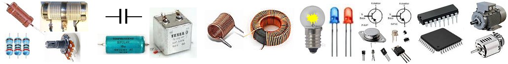 |
| Resistors and potentiometers Capacitors Solenoid and toroidal coils Light bulbs and LEDs Transistors Integrated circuits Electric motors |
Electrical circuits
Note :
For the basic electronic components of resistors, capacitors and
coils, when analyzing the properties of electrical circuits, we
will assume that these are ideal components - resistors with
resistance R, capacitors with capacitance C and
coils with inductance L.
In order to use the properties of
these electronic components, we must connect them
conductively to each other in an electrical circuit
so that an electric current can pass through them. If the
conductive path is not nterrupted in the electrical circuit, it
is a closed electrical circuit. If this
conductive path is interrupted at some point, it is an open
electrical circuit. The simplest method here is an
electro-mechanical switch whose contacts can be turned on -
connected or turned off - disconnected. More complex electronic
methods of closing and opening electrical circuits and their
parts are also used.
The basic parameter of an
electrical circuit (and of each electrical component) is its volt-ampere
characteristic - the dependence of the current I
on the supply voltage U. In the simplest situations in
practice, this dependence is linear according to Ohm's
law I = U/R, where R is the total resistance that the
individual components in the circuit offer to the electric
current. This is the resistance that a conductor offers to
flowing electrons. The unit of electrical resistance is 1 Ohm
[?]. A current of 1 A flows through a circuit or element with a
resistance of 1? at a voltage of 1 V. In a series connection, the
values ??of the individual resistances are simply arithmetically
added, in a parallel connection, their inverse values are added.
For semiconductor components - diodes, transistors - Ohm's law
does not apply exactly, the volt-ampere characteristic is more
complex, nonlinear. Common metal conductors, such as copper wire,
have a very small resistance of the order of milli?/meter, so it
is neglected in practical electronics. Superconducting
materials actually have almost zero resistance (see
"....." in §,,,,,,....). Non-conducting
substances - dielectrics - do not contain free charge carriers
and, on the contrary, have an infinite specific resistance.
The situation is more complicated
in electric circuits with alternating current, usually
with a harmonic sinusoidal waveform in time t with
frequency f : I = I0.sin (2p.f.t). Ordinary resistors behave
almost the same as in direct current, their ohmic resistance does
not depend on frequency. However, capacitors and coils
behave completely differently. In a DC circuit, a
parallel-connected capacitor can be charged once. If it is
connected in series, it also charges once, but its dielectric gap
is non-conductive and the circuit behaves as if it were disconnected,
no current flows. In a DC circuit, on the contrary, an electric
coil behaves like a conductor. However, with alternating voltage,
the capacitor electrodes alternately charge, discharge and then
charge with opposite polarity, which makes the capacitors
effectively conductive for alternating current (the insulation gap of the
capacitor is overcome by the so-called Maxwell displacement
current, discussed below "..."). The effective resistance of the
capacitor (capacitance) to alternating voltage is indirectly
proportional to the capacity C of the capacitor and
indirectly proportional to the frequency f :
XC = 1/2p f . C . In an electric coil, the
alternating current inside creates a variable magnetic field,
which in turn induces an electric voltage that opposes
the supply voltage - self-induction occurs. The effective
resistance of the induction coil (inductance) to alternating
voltage is directly proportional to the inductance L of
the coil and directly proportional to the frequency f :
XL =L.2p.f .
The effective resistance of the
capacitor XC and the inductance XL to the alternating voltage is called impedance (lat. impedire = to hinder, to
be in the way, to hold back, to hinder, usually marked with X). Also "reactive"
resistance or "reactance", while the
resistance of the resistor R is called "active
resistance". Ohmic resistances + capacitance and
inductance are then added to the resulting impedance of the
circuit Z. When quantifying impedances, the circular
frequency w = 2p f is more often used rather than the
frequency f. The capacitive impedance XC = 1/w . C , the inductive impedance XL = w . L and the active resistance R of
the resistor are not added together arithmetically (as is the
case with a resistor) in an electrical circuit, but "geometrically".
The impedance of a series connection of a resistor R with
a capacitor C is Z = Ö[R2 -
1/(w.C)2], for a parallel connection of a resistor
with a capacitor the resulting impedance is Z = Ö(R2+w2C2R4)/(w2 C.R2 +1) .
When alternating current passes
through a resistor, the sinusoids of voltage U=U0.sin (w.t) and current I=I0.sin (w.t) are in phase with each other, the
voltage and current reach their minimum and maximum at the same
time instants. However, when alternating current passes through
capacitors or inductors, a phase shift j occurs between the voltage and current -
the voltage and current reach their maximum or minimum at
different times. If we assign an angle of 360° to one whole
period, then on the capacitor the voltage lags behind
the current by 90° - this is caused by the process of
alternating charging of the capacitor. On the other hand, on the
inductor the voltage leads the current by 90° - due to
self-induction.
 |
| Phase relationship of alternating voltage U and current I for a resistor, capacitor and coil. | Phase diagram of impedance of resistor R and reactance X |
If resistors, capacitors and
coils are connected in a circuit, the total phase shift between
voltage and current will vary depending on the ratio of the
values of R, C and L of these components. In
a series-connected RLC circuit of "ideal"
components of resistor, capacitor and coil, 3 significant cases
can occur :
1. If XL < XC , the voltage on the inductor
will be less than that on the capacitor and the RLC circuit will
have a capacitive character - the voltage will lag the current by
0<j<-90°.
2. If XL > XC , the voltage on the coil will
be greater than that on the capacitor and the RLC circuit will
have an inductive character - the voltage will lead the current
by 0<j<90°.
3. In the special case XL = XC, the coil will have the same
voltage as the capacitor and the RLC circuit will have only a
resistive character, the total phase shift will be j = 0. This special state occurs at a very
specific resonant frequency f = 1/2p.Ö(L.C) .
The total effective impedance of the circuit is Z = Ö[R2 + (w . L)2 - 1/(w.C)2] and the phase shift between the total
voltage U and the current I is j = arccos R/Ö[R2+(XL-XC)2] .
During the rotational movement of
a point around a circle of radius r, its horizontal and
vertical coordinates x,y take on the values x = r.cos j and y = r.sin j ,
where j is the angle between the line connecting
the origin of the coordinates (0,0) and the position (x,y) of the
point on the circle. Therefore, the alternating voltage/current
U/I = U0/I0.sin 2pf.t is often represented by a circularly
rotating vector U/I (0,U0/I0) of length |U0/I0| rotating with angular velocity j(t) = 2pf.t =
w.t. This vector is
sometimes called a "phasor", since its
rotation j gives the instantaneous phase of
the alternating voltage.
Impedance is sometimes expressed
in a complex (imaginary) formalism. The complex
expression of impedance in algebraic form is Z = R + i.X, where R
is the "effective" resistance, X is the
impedance, and "i" is an imaginary unit. These two
numbers R and X can be plotted graphically as a
point (R,X) in the two-dimensional plane of complex numbers,
where the horizontal axis has the real coordinates of R
and the vertical axis has the imaginary coordinates of X.
Each complex number can then be represented by a vector in this
plane, starting at the origin (0,0) and ending at the point
(R,X). This vector can also be expressed by its length |Z|
= Ö(R2 + X2) and the value of the angle j = arctang(X/R) that it makes with the
horizontal axis. It is therefore a complex-expressed
"phasor". This results in a phase diagram
showing the complex impedance Z plotted as a vector in the
complex plane, which has the real component of the impedance as
the horizontal coordinate and the imaginary component of the
impedance as the vertical coordinate. The impedance can then be
expressed in the trigonometric form of the complex
number Z = |Z| . (cos
j + i . sin j), which is sometimes written in
the exponential form Z = |Z| . e i . j.
This formalism has the advantage
that the same resulting relations apply to the
"addition" of impedances as to the addition of DC
resistances. However, a certain disadvantage is less intuitive
clarity, since imaginary numbers are only model and artificial,
they do not occur in real nature. The complex formalism for
impedance is used more by electronics experts in the design and
analysis of more complex RLC circuits.
Favorized
sinusoids !
The functional course of the time dependence of
electromagnetic signals can be very different in principle.
However, when we observe electrical signals in various circuits,
alternating voltage, radiation of electromagnetic waves and their
reception, we observe in the vast majority a harmonic
sinusoidal course, exact or at least approximate. It may
be interesting to discuss what favors sine waves over
other mathematical functions..?..
From a mathematical point of
view, the sine or cosine function has a "gift of special
resisllience": when we differentiate it d sin(x)/dx = cos(x) we get cosine, which is
again a sine with a phase shift of 90°. Even after integrating nsin(x)dx = -cos(x) it is just a negative
cosine. Multiplying the sine wave by a constant will again make
it a sine wave. The projection of a circular motion of radius r
into the coordinates x and y oscillates harmonically as x(t) = r . cos w.t , y(t) = r . sin w.t ,
where w is the angular frequency.
All oscillatory movements caused
by a force F which is proportional to the deviation x
from the equilibrium state F = -k.x -
the movement of a classical pendulum, waves on the water surface,
elastic oscillations of particles in a material environment,
electrical oscillations in an LC oscillator - occur with a
resulting deflection of the form x(t) = r . sin w.t . From an electronic point of view, a
sinusoidal signal is the only shape that does not change its
character when it passes through an electrical circuit containing
capacitances, inductances and resistors. And each configuration
of an electrical signal or electromagnetic wave can be decomposed
using Fourier analysis into a superposition of
a smaller or larger number of harmonic sinusoidal signals or
waves of different frequencies and amplitudes..!.. Any
nonlinearity in an electrical circuit distorts the pure
sinusoidal waveform, which is manifested by the appearance of
signals of the so-called higher harmonics, which again
behave as sinusoids of different frequencies.
Sine oscillations and waves are
naturally produced by nature in the field of mechanics
and electrodynamics; similarly to the field of gravity in the
universe, elliptical paths of movement of planets around stars,
orbits of moons around planets, or mutual orbits of stars in
binary and multiple stellar systems arise naturally. Sinusoids
and cosinusoids are therefore natural functions that can be used
to model and quantify a number of processes in nature using
simple harmonic oscillators.
The vast majority of electrical
energy for the world economy and consumption in our homes is
produced in alternators, where a rotating magnetic field induces
an alternating current in coils of exactly
sinusoidal form with frequency of 50 or 60 Hz.
How fast
is electricity ?
In terms of speed, we encounter two extremes in electricity:
the speed of propagation of the electromagnetic field and the
speed of movement of electrons in conductors. It is a notorious
experience that when we turn on the switch, light bulbs many
meters away (even
kilometers - city lighting) immediately light up. Or a telephone
connection even over long distances is immediately established (we do not consider complex relay
connections here).
So one could conclude from this that the electrons are moving at
a high speed in the conductor. This conclusion would be
completely wrong.
Although the electrons in the conductor,
even without the electrical circuit switched on, move at room
temperature at very high speeds of the order of thousands of
km/s., however, these are only microscopic completely chaotic
thermal movements that in total do not create any electric
current. When we apply a voltage to the conductor, in addition to
their chaotic movement, they begin to move slowly in one
direction, towards the positive voltage - the so-called drift
movement. However, the speed of this movement is very small, on
the order of millimeters/second. So how come the remote lightbulb
lights up immediately? When the switch is turned on, the
electrons almost immediately begin to move along the entire
length of the connecting wire, and the bulb lights up
immediately. That practically instantaneous effect is caused by
the speed of propagation of the electromagnetic field along the
conductor, which is close to the speed of light (see below "Speed of propagation of an electromagnetic
signal").
So "snails activated at the speed of light"....
The
movement of electric charges in space and time is generally
described in field theory using the current density j(x,
y, z, t) º r . v , where v
is the instantaneous velocity of charges at that point (x, y, z);
electric current flowing through a given surface S then I
= S òò j dS. The law
of conservation of electric charge then states that the
change in charge contained in each given spatial area V
must be equal to the amount of charge that passes through the
closed surface S = ¶V surrounding this area :
 |
(1.31a) |
Using Gauss's theorem, the well-known equation of continuity follows
| div j + ¶r / ¶ t = 0 , | (1.31b) |
expressing the law of conservation of electric charge in differential form.
Coulomb's law of
excitation of the electric field by charges
The
fundamental law of electricity is Coulomb's law
of excitation of an electric field by electric charges (in the previous §1.4 we stated
it under the number (1.20b)) :
| q l . q 2 Fel = - k . ------------ . r° , r2 |
(1.20b) |
| Fel = - k . q1 .q2 /r2 . r° , | (1.20b) |
which expresses the
mutual force action of two (point) electric charges q1 and q2 placed in a vacuum at a distance r
from each other (r°
is the unit position vector of both charges relative to each
other). The
"-" sign expresses the fact that charges of the same
name (same polarity) repel each other. The value of the constant k
depends on the system of units used. In fundamental physics, k=1
is declared (which
naturally defines the unit of electric charge by its force action
per unit distance *),
in the SI system k = ~8.988×10⁹ N m2 C-2 and the unit of electric charge is 1
Coulomb (C).
*) Unfortunately,
the historical development of physics has led to the fact that in
the SI system of units, charge is not primarily quantified by its
electric force effects, but only indirectly by the magnetic
effects of electric current (the unit of current is Ampere;
one Coulomb is then defined as 1A/1s).
In the SI
system, Coulomb's law is written in the form with coefficient k =
1/4pe0 :
| Fel = - 1/4pe0 . q1 .q2 /r2 . r° , | (1.20b) | S I |
where e0 is the permittivity of
vacuum e0 = ~8.854×10⁻¹² F.m-1. The permittivity of material media will
be discussed below - "Coulomb's law in material media".
Etymology:
Lat. permittere = to forward, to allow - to what extent
the material media allows electric forces to penetrate.
For the action of force in space
"at a distance", physics introduces the concept of a physical
field, which is a space in which forces of
a given type act on (test) particles. In electricity, it
is an electric field excited by electric charges
(and also by
electromagnetic induction). If the electric charges do not move, it
is an electrostatic field that is quantified by the electric
intensity vector Eel, which is the force acting on a unit test
charge q, i.e.
| Fel = q . Eel . |
The electric force and
intensity Ee are generally a function
of the location - coordinates in the studied space. For the
sake of brevity of notation, instead of the individual
coordinates x,y,z, we will use the position vector r
(radius vector) - the line connecting the origin of the
coordinate system and the investigated point, where, for example,
the charge is located or where we determine the intensities E(r)
and potentials j(r) of the
fields.
In addition to the intensity Eel
, the electric potential j is also introduced in the electric field.
It is a scalar quantity describing the potential energy
of an electric charge in an electric field - the amount of work
required to transfer a unit electric charge from a reference
(default) point, where the potential is considered to be zero, to
a given point r in the electric field.
The reference point with zero potential is usually taken to be a
point infinitely distant from the system of charges, where no
electric field is acting (at least in the limit); in practice, the surface of the
Earth (grounding) is taken. The potential j of an electric field is related to its
intensity E by the relation
| Eel = - grad j(r) , |
where grad f
= [¶f/¶x, ¶f/¶y, ¶f/¶z] is a vector differential operator
quantifying the "steepness of the slope" - gradient
- of the scalar field f in the direction of the
coordinates x,y,z.
The potential difference of two
points gives the electric voltage U
between these two points, the unit of which is 1 volt [V]. A
voltage of 1 Volt is such that, in order to overcome it by a
point charge of 1 Coulomb, it is necessary to perform (or release - depending on the
polarity) work of 1
Joule. The voltage U between two points r1 and r2 in an electric field of
intensity E(r) is given by the difference
| Ur1,r2 = j(r2) - j(r1) = r1nr2 E(r) . dl |
(integrated along the
line "l" between the two points). In practice, the electric
voltage is quantified not so much for different points in space,
but between the electrodes to which it is supplied from
a certain source. When a charge q is moved between points
with a voltage difference U, work is performed (or
released) W = q . U.
Coulomb's law can then be
expressed in terms of the electric field intensity Eel (we will omit the index "el" in
the following)
excited in space around a point electric charge Q :
| E = k . Q / r2 . r° . | (1.20c) |
The excited electric potential here is then
| j (r) = k . Q / | r | . | (1.20d) |
The potential depends
only on the distance |r|, not on the direction
relative to the exciting charge Q.
In practice, the electric field
is usually excited not by randomly distributed electric charges,
but by electrodes to which an electric voltage [V] is
applied from a suitable source, which can be a galvanic cell, an
electro-mechanical generator, an electronic circuit, or other
device or material configurations.
Electric
field in a material environment
Coulomb's law in the form (1.20b) also applies not only in
vacuum, but in an electrically homogeneous and isotropic material
medium called a dielectric
| Fel = - 1/4pe . q1 .q2 /r2 . r° , | (1.20b´) | S I |
while the
proportionality constant k expressed in the form k = 1/4pe, where e is the permittivity (dielectric
constant) of the given material medium. The permittivity of a
vacuum is e0 = ~8,854×10-12 F . m-1 .
The names "insulator"
and "dielectric" are sometimes terminologically
distinguished (a dielectric is an insulator in which particles
are polarized). Due to the atomic structure of all known
substances, polarization of atoms and molecules always occurs, so
from a physical point of view the terminological difference is
irelevant.
There are basically two types of
dielectrics. Either the substance is composed of polar atoms
or molecules - permanent dipoles, which rotate in the direction
of the field under the influence of an external electric field.
Or the substance is composed of originally non-polar particles,
which are, however, polarizable under the influence of
an external field. In both cases, polarization occurs when placed
in an electric field, with the polarized dipoles acting
against the external field and polarization reducing
the resulting intensity E of the electric field
in the dielectric compared to the field in a vacuum.
The way in which the electrical
polarization and magnetization of atoms and molecules of the
material environment arise and how it is reflected in the
intensities of the resulting electric and magnetic field is
clearly shown in §1.1, passage "Electromagnetic and
Optical Properties of Substances" monograph "Nuclear Physics and Ionizing Radiation
Physics".
The permittivity of materials e is often quantified using the relative
permittivity er = e/e0, also called the dielectric
constant. It indicates how many times the electric force between
charges decreases when they are placed in a given medium instead
of a vacuum (at the
same time it indicates how many times the capacitance of a
capacitor increases when a dielectric is inserted between the
plate electrodes).
For vacuum, of course, er = 1, for air and other dilute gases it is
also close to 1. For wood and pressed paper, er is ~2-2.5, for plexiglass about 3.5, for
water ice 4.8, for diamond 5.5, for water er =80 (it is a polar compound).
For our theoretical analysis of
the nature of electrical phenomena, we do not need to introduce
the quantity D =e . E called electrical
induction. We will only use it below for the formulation of
Maxwell's equations in a material environment (1.38´-41´).
In a vacuum, the dependence
between the size of electric charges and the excited electric
field is exactly linear (direct proportionality) with a
coefficient of 1/4pe0 up to colossally high intensities of
about 1012 Volt/micrometer. It is limited
to the quantum level (brief
discussion "What is the
strongest electric field?"). In a dielectric material environment
under normal situations, this linearity is also preserved, only
with a somewhat lower coefficient of 1/4pe.
Linearity here can be disturbed only for very strong
electric fields, when the phenomenon of the dielectric's
electrical strength can manifest itself :
At a high value of the electric
field intensity, the insulating properties of the dielectric can
be violated - an electrical breakdown and an
avalanche-like passage of a large number of charged particles
(mostly electrons) can occur, and a spark can jump
between the electrodes of opposite polarity. Under the influence
of a strong electric field, the originally bound electrons are
released and can accelerate so much that in collisions with
neutral atoms and molecules, more and more electrons are ejected,
which creates an avalanche-like current, an electrical breakdown,
within a few nanoseconds. If the electrodes are powered by a
"harder" electrical source of greater power, a more permanent
discharge can occur at the breakdown point - an electric
arc, with thermal effects of melting or igniting the material.
The value of the breakdown voltage [kV/mm] depends
primarily on the type of insulating (dielectric) material, but
also on the configuration of the electrodes, on the possible
content of impurities, microscopic dislocations and free
electrons or ions, which are also contained in trace amounts in
insulators. For air it is about 2-3 kV/mm, for glass and
porcelain about 10-30, for PVC 30-50, polyethylene about 100, for
polyester up to 180 kV/mm.
In addition to classical
dielectrics, which are polarized by an external electric field
and disappear after the field is removed, there are a few rare
materials that can be permanently polarized even after
the external electric field is removed - so-called electrets,
electrical analogs of permanent magnets. The basic method of
creating an electret consists of three steps: 1.
Melting a suitable dielectric substance, e.g. paraffin
or resin. 2 Inserting the molten substance into
a strong electric field - between electrodes to which a
high voltage of several kilovolts/cm is applied. Here, the atoms
or molecules inside the molten substance are polarized. 3.
Allowing the molten substance to cool and solidify in
this electric field. The polarized molecules in the solidified
substance lose mobility ("freeze") and retain their polarization even after
the electric field is turned off. An electrostatic field will
then be permanently active around the electret. Weak electrets
also occur naturally in nature, mainly in various forms of
silicon oxide. For artificially produced electrets, some easily
meltable dielectric materials are suitable, such as paraffin
(wax), resins, polymerized plastics such as fluoropolymers,
polypropylene, PET, PTFE, and sulfur, ...... In addition to the thermal
method, electrets are more recently prepared by corona
discharge, irradiation of thin layers with soft X-rays,
injection of electrons using an accelerator. Electrets
are used electromechanically in small electret microphones, in sensor
transducers in movement and deformation monitors, air filtration
media, xerography, memory devices, integral detectors of ionizing
radiation (especially
when measuring radon concentration)...
From the point of view of field
theory, Coulomb's law can be expressed in the form of Gauss's
theorem of electrostatics (Fig. 1.3a)
 |
(1.32a) |
from which the differential equation follows
| div E = 4p r . | (1.32b) |

Fig.1.3. Excitation of electric and magnetic fields by electric
charges and currents.
a ) The total electric charge Q contained in the
space inside any closed surface S is given by the Gauss
theorem flux of the electric field E over the closed
surface S .
b ) Circulation of the vector magnetic field B
around the closed curve C is proportional to the total
electric current I flowing through the surface S bounded
by the curve C .
c ) The electromagnetic field excited by a
system of moving electric charges is given by the distribution of
charges and currents, retarded always by the time required by the
field to overcome the distance r - r' from the
individual places dV' of the system to the examined place r
.
In nature and in
electronic applications may arise even strong electric fields at
a volage of several millions of volts. For interest, we can give
a small discussion, what is the strongest electric field that can
be achieved? :
What
is the strongest electric field can be ?
In classical (non-quantum) physics, the electric field in a
vacuum can be arbitrarily strong, almost to infinity (in a material environment,
however, this is limited by the electrical strength of the
dielectric) . From
the point of view of quantum electrodynamics , however,
even in vacuum there is a fundamental limitation caused by the
existence of mutual antiparticles of electron
and positron : it is not possible to create an
electric field with an intensity stronger than E e-e+
= m e2 c3 / e.h = 1.32 × 10¹⁶ V/cm, where me is the rest mass of the electron or
positron. When this intensity is exceeded, the potential gradient
is higher than the threshold energy 2me c2 and a pair of electrons and
positrons is formed, which automatically reduces the
intensity of the electric field. Such a strong electric field has
not yet been created, with conventional electronics this is not
possible; strong impulses from extremely powerful lasers could be
a certain possibility in the future ...
At the end of §1.6, in the
passage "Nonlinear electrodynamics", a purely hypotetical
model of classical relativistic nonlinear electrodynamics will be
discussed.
Magnetic field excitation
In addition to the electric forces acting even between
stationary charges, there are also magnetic forces
acting only between moving charges in the field of
electricity. The space in which these forces act is called a magnetic
field. If an electric charge q moves in this
space with a velocity v, it is acted upon by a
force
| Fmag = q . [ v x B ] , | (1.30b) |
where B
is the magnetic field intensity (for
historical reasons called magnetic induction), "x" means the vector product. It is
called the Lorentz force. This force is perpendicular
to the direction of the velocity v of the
particle. The SI unit of magnetic induction B is 1 Tesla:
In a homogeneous magnetic field of intensity (induction) of 1
Tesla, a linear conductor of length 1 meter, stretched
perpendicular to the magnetic field lines and flowing with a
constant current of 1 Ampere, exerts a force of 1 Newton. In the
CGS system, the unit of magnetic induction is 1 Gauss =
10-4 Tesla.
The magnetic field
is excited by moving electric charges, ie electric
current, according to the Biot-Savart-Laplace law.
The basic form for a point electric charge Q, moving with
a velocity v, gives how strong the
magnetic field B will be at a distance r
- at a location with a position vector r = r . r0 :
| B (r) = k . Q . [v x r0] / r 2 . | (1.33a) |
The Biot-Savart law is usually formulated in differential form for an electric current flowing through a linear conductor :
| d B = k . I . [dl x r0] / r 2 , | (1.33b) |
where dl is an element of the length of the conductor through which a stationary electric current I flows, r is the distance of the measured location, and r° is the unit position vector pointing from this current element to the investigated location ("x" is the vector product). The value of the constant k depends on the system of units used. In fundamental physics, k=1 is declared, in the SI system it is k= m0/4p, where the coefficient m0 is the permeability of vacuum, in SI units it is m0 = ~1,257×10-6 N . A-1 :
| B (r) = m0/4p . Q . [v x r0] / r 2 . | (1.33a) | S I |
| d B = m0/4p . I . [dl x r0] / r 2 , | (1.33b) | S I |
Etymology:
Lat. permeare = to pass through, to let through - here
the property of a substance to let through or amplify a magnetic
field.
The permittivity e0 and permeability m0 are related to the speed of
light c in vacuum by the relation c = 1/Ö(e0.m0), as will be shown in the section "Electromagnetic waves". From the comparison of
relations (1.30b) with (1.33a,b) we see that magnetism is
inextricably linked to the dynamics of the movement of
electric charges: The magnetic field exerts a force on
moving charges and is also created by the movement of charges.
From relation (1.34a,b) it is then seen that a magnetic field can
also be created by a time-varying electric field.
Magnetic field in a material
environment
The Biot-Savart-Laplace law of excitation of a magnetic field in
the form (1.33a,b) is valid not only in a vacuum, but also in a
homogeneous and isotropic material environment, where
the permeability of the vacuum m0 is replaced by the magnetic permeability
of the given material m. Most substances (gases, water, dia- and paramagnetic
metals such as copper, aluminum, gold, .... ) have permeability almost equal
to m0; only the ferromagnetic metals iron,
cobalt, nickel and their alloys have permeability on the order of
100× to 100000 times higher.
For materials, the relative
permeability mr = m
/ m0 compared to vacuum is
introduced, according to which materials are divided into 3
categories :
-> Diamagnetic
mr < 1, which slightly weaken the magnetic
field. The inner shells in the atomic shell are fully occupied by
electrons, the orbital and spin moments are completely
compensated, the resulting magnetic moments of the atoms are
zero. When a magnetic field is excited, a weak magnetic moment is
induced in the material, acting against the external
magnetic field. These are some metals such as copper, silver,
gold, mercury, most organic substances, water, inert gases.
-> Paramagnetic
mr > 1, which slightly strengthen the
magnetic field. The inner shells in the atomic shell are not
fully occupied by electrons, the magnetic moments of the atoms
are not zero, but are irregularly oriented in all directions.
After the external magnetic field is excited, the moments of the
atoms are oriented in the direction of the external field, which
slightly strengthens the resulting magnetic field. These
are, for example: metals aluminum, magnesium, chromium, platinum
...
-> Ferromagnetic
mr >> 1, which significantly enhance
the magnetic field. This is due to the fact that these substances
contain spontaneously arising magnetic domains, which
have their magnetic moments oriented identically. Without the
presence of an external magnetic field, the directions of the
individual domains are chaotically oriented, so the resulting
magnetic moment is zero. However, it is enough to excite a
relatively weak magnetic field for the magnetic moment of the
domains to orient in the direction of the external field, which
leads to a significant amplification of the external
magnetic field. These are mainly iron, cobalt, nickel,
gadolinium, ruthenium and their alloys (such as permalloy
20% Fe, 80% Ni - mr~100,000; suprrmalloy 20% Fe, 75%
Ni, 5% Mo - mr~800,000). Ferromagnetic properties only
work at sufficiently low temperatures. At temperatures higher
than the so-called Curie point, the magnetic domains
disappear and the material changes from a ferromagnetic to a
paramagnetic state. For iron, the Curie temperature is 1040 oC,
for neodymium magnets only about 70-120 oC.
However, in very strong external
magnetic fields, almost all domains are already oriented in the
direction of the field and further increase in its intensity
leads only to a milder paramagnetic enhancement. The
ferromagnetic enhancement of the external field is therefore dependent
on the intensity of the external field, showing a saturation
state.
 |
| Left: Magnetization dependences for basic categories of substances. Right: Hysteresis loop of ferromagnetic materials. |
Magnetization
characteristics - the dependence of the resulting magnetic
induction on the excitation intensity - are linear straight
lines for dia- and paramagnetic materials, because theirmr is constant. For ferromagnetic materials,
it is no longer a straight line, because their mr changes during magnetization depending on
the intensity of the magnetic field. A relatively complex
magnetization characteristic is manifested here, showing a saturation
state BS .
In addition, a number of
ferromagnetic materials exhibit a special dynamic
"memory" behavior called hysteresis -
irreversibility of magnetization processes. If we excite a
sufficiently strong magnetization, when the excited magnetic
field is reduced again, the resulting magnetization curve does
not return to the same functional dependence as before when
increasing, but has somewhat higher values than before. When the
intensity of the magnetic excitation drops to zero, a certain
non-zero remanent magnetic induction Br
remains, which the material retains (approximately 0.1-1 T). Part
of the magnetic domains remains oriented. To cancel the remanent
magnetization, it is necessary to apply a certain coercive
magnetization of the opposite direction, the further increase of
which then leads to a magnetization curve of the opposite
polarity, also showing the saturation state -BS. When
alternating magnetization in opposite polarities, a closed curve
is created, called a hysteresis loop.
According to the width of the
hysteresis loop, ferromagnetic materials are divided into two
categories :
--» Magnetically soft have
a narrow hysteresis curve with a low Br value, so that
after the external magnetic field is removed, their own magnetic
field also practically disappears. This property is possessed by
pure iron (with a
low carbon content <0.1%), permalloy.... .. ......
--» Magnetically hard with
a wide hysteresis loop and a large Br value. After the
external magnetic field is removed, they remain magnetized and
behave like a permanent magnet. Their magnetic field can
be removed by an external magnetic field of opposite polarity.
This is how iron-steel with a high carbon content, tungsten
steel, chromium and cobalt behave. The strongest permanent
magnets are prepared from the rare earth elements samarium
(Sm-Co-5, Sm-2-Co-17) and neodymium (Fe-Nd-B). They achieve high
remanence values Br ~ 0.8-1.4 Tesla.
For our theoretical analysis of
the nature of magnetic phenomena, we do not need to introduce the
quantity H =e . B called magnetic
intensity. We will only use it below for the formulation of
Maxwell's equations in a material environment (1.38´-41´).
From the Biot-Savart's law
(1.33b) follows the Ampere's law
 |
(1.33b) |
according to which the curve integral - circulation - of the magnetic induction vector along any closed curve C is proportional to the total current flowing through the surface S , which this curve surrounds (Fig.1.3b).
The integral on the left side of Ampere's law depends only on the curve C = ¶S, so for equation (1.33b) to be generally valid, the area integral on the right side must be the same for all surfaces S having the curve C behind the contour. Using Gauss sentences can be easily shown that this is only fulfilled if div j = 0, i.e. when it is the stationary electric current that does not cause changes in the distribution of electric charge in the vicinity of the curve C. For general non-stationary currents, it is therefore necessary to generalize Equation (1.33b) to be compatible with the continuity equation. Substituting in the equation of continuity (1.31b), which also applies to non-stationary currents, for r from equation (1.32b), we get
div [ j + (1/4p) ¶E / ¶t] = 0 .
This vector is found, j + 1/4 p ¶E / ¶T whose divergence is always equal to zero, and that in the stationary case, coincides with a normal density "conductive" stream j. The expression jMaxw = (1/4p) ¶E/¶t is called the Maxwell displacement current and can exist even in a vacuum without the presence of real electric charges. Maxwell proposed in the case of a non-stationary field in equation (1.33b) to replace the current density j with the vector j + (1/4p) ¶E/¶t , or stated the hypothesis that the displacement current has the same magnetic effects as the normal "conductive" current of real electric charges :
| (1.34a) |
The magnetic field is thus excited by the total effective current
| Ief = nn j dS
+ nn (1/4p) ¶E/¶t dS . conductive current Maxwell displacement current |
(1.35) |
This Maxwell's hypothesis proved to be very correct and fully corresponds to all experiences with electromagnetic phenomena. The Maxwell displacement current is, for example, that current which "overcomes" the insulating layer of capacitors and causes their "conductivity" for alternating currents. If we have a planar capacitor with a plate surface S , then between the intensity of the homogeneous electric field in the gap and the charge of the capacitor q, the relation E = 4p q/S holds, so that the instantaneous current flowing through the capacitor I = ¶q/¶t = S. (1 /4p) ¶E/¶ t = S. jMaxw is given by Maxwell current.
The displacement current, which - although not formed by the motion of real electric charges - has normal magnetic effects, finds its analogy in the gravitational field, where even in a vacuum without real material bodies there is effective Isaacson energy and momentum of gravitational wave, which has gravitational effects (curves spacetime) like any other matter (see §2.7-2.8).
By converting the integral along the curve C using the Stokes theorem to the integral over the surface S surrounded by this curve, we obtain the equation of excitation of the magnetic field by an electric current (conductive and displacement) in a differential form
| rot B = (4p/c) j + (1/c) ¶E / ¶t . | (1.34.b) |
From this equation it is
clear that the magnetic field can be created not only by the
movement (current) of electric charges, but also by a time-varying
electric field .
Note:
Note the coefficient 1/c = 3.33×10⁻⁹ s/m
in all relations (1.33)-(1.34) between the magnetic field
intensity B, the current I, j
and the electric field E. The very low value of
this coefficient reflects the fact that the magnetic
field arising from the motion of charges or
electromagnetic induction is generally very weak
compared to the electric field (excited by the same charges). For electromagnetic waves, this
fact is briefly discussed below in the passage "Lesser-known properties of electromagnetic
waves".
A strong magnetic field of tens
of Tesla can be created in the laboratory by passing a strong
current of several thousand Amperes through electromagnetic
coils, mostly superconducting (§1.5, section "Electromagnets in accelerators" and §1.3, section "Tokamak"). In the universe, powerful
magnetic fields arise during the gravitational contraction and
collapse of compact stellar objects such as white dwarfs and
neutron stars, when the acceleration of rotation under
the law of conservation of angular momentum enormously thickens
the magnetic field lines and the magnetic field can increase to
enormous values of up to ~108-1012 Tesla (§4.2, section "Astrophysical significance of
supernovae").
Another basic law of electromagnetism is the finding that magnetic field lines are continuous and closed curves. In other words, the magnetic field is source-free, there are no magnetic "charges" (monopolies) *) from which magnetic field lines originate or enter (unlike electric charges, where electric field lines begin and end). Therefore, exactly as many magnetic field lines must enter from the closed surface S as enter them, ie the magnetic flux from the closed surface is equal to zero :
 |
(1.36a) |
By converting the area integral to the volume integral using the Gauss theorem, we get the equation
| div B = 0 , | (1.36b) |
which is a mathematical
expression of the principle of continuity of magnetic field lines
in differential form.
*) We
leave aside here the Dirac's hypothesis about of magnetic
monopoles, based on the formal requirement of symmetry of
the equations of electrodynamics. Experiments trying to find
magnetic monopoles have not yet yielded any results. However,
magnetic monopoles are considered in quantum unitary field
theories and their possible significance for the cosmology of the
very early universe is also discussed (§5.5 "Microphysics and Cosmology. The
Inflationary Universe.").
Electromagnetic induction
The generation of an electric field by a time-varying magnetic
field is expressed by Faraday's law of electromagnetic
induction
 |
(1.37a) |
according to which the electromotive force (voltage) U s ?nC E dl induced along a closed curve C is proportional to the speed with which a change in magnetic flux F s nnSB dS by surface S enveloped by the curve C. In the integral on the right side it does not matter the choice of the surface S surrounded by the given curve C , because the magnetic field is source-free (div B = 0). By converting the curve integral on the left side using the Stokes theorem to the area integral we get the law of electromagnetic induction expressed in differential form :
| rot E = - (1/c) ¶B / ¶t . | (1.37b) |
Maxwell's
equations
The
outlined application of the mathematical apparatus of
differential and integral calculus to the empirically determined
laws of electromagnetism (ie to the knowledge of Coulomb, Ampere,
Faraday, Biot, Savart, etc.) and their generalization was
performed by J.C.Maxwell, who arrived at a complete system of
basic equations of the electromagnetic field and summarized the
individual findings into a comprehensive theory. J.C.Maxwell
formulated his very important equations in 1865, first in the coordinate
form of the components x,y,z of the electric E
and magnetic B fields and the current density j.
This resulted in a quite complex system of more than 20 equations
(sometimes a also complex
so-called tetrad formalism is mentioned, but it was soon
abandoned). They
were reformulated in the compact vector form
(1.38)-(1.41) by J.W.Gibbs and O.Heaviside around 1884.
These Maxwell's equations (1.31b) to
(1.37b), which we gradually derived above, can be clearly
summarized in differential form as follows :
| Maxwell's equations of the electromagnetic field |
 |
(1.38) |
| (1.39) | |
| (1.40) | |
| (1.41) |
 |
(1.38) | S I |
| (1.39) | ||
| (1.40) | ||
| (1.41) |
These equations
determine the electric and magnetic fields E and B
excited by a given distribution of charges and currents r and j. The first pair
of Maxwell's equations describes the generation
of electric and magnetic fields by material sources, ie the
density of electric charge r and current j protruding
on the right side; the second pair expresses
other internal properties of the field. It can
be seen from equations (1.38) and (1.40), that the electric E
and magnetic B fields can mutually generate
each other with their time variability --> electrodynamics
.
The
Lagrangian for the electromagnetic field
We derived the Maxwell equation of the electromagnetic field here
physically - inductively from Coulomb's,
Biot-Savart's, Ampere's, Faraday's law. In theoretical physics,
the laws of motion and field equations are often derived in a
deductive manner using the variational principle of least
action [165]. The classical physical system is described
by the integral of the action S
| S = ò L (q1 , q2 , ... qn ,, q.1 , q.2 , ......... q.n ) d t .... |
where L is the
so-called Lagrange function - Lagrangian,
describing all dynamic characteristics qi of a given system and their time
derivatives q.i , n is the number of degrees of
freedom. The variational principle of the smallest action dS = 0 then leads to Lagrange's
equations, from which the equations of motion
or field equations of the studied system follow (for more details, see §2.5 in
the section "Variational Derivation of
Gravitational Field Equations") .
For the electromagnetic field, the Lagrangian has the form:
| L = 1/8p ( E 2 - B 2 ) + j . A - r . j . | (1.42) |
Maxwell's equations (1.38-41) can be derived from the variational principle of the smallest action with Lagrangian (1.42).
Electromagnetic field in the
material environment - electrodynamics of the
continuum
In our theoretical analysis, we consider the
electromagnetic field mainly in vacuum, which is
the basic natural environment for fundamental physics. For the
sake of completeness, we will briefly outline here how the
electromagnetic field behaves in material environments
(the material "continuum"). The interaction of
electric and magnetic fields with atoms and molecules of matter
leads to their electric polarization and magnetization,
which is reflected in the vectors of electric and magnetic field
intensity. The way in which the electrical polarization and
magnetization of atoms and molecules of the material environment
arise and how it is reflected in the intensities of the resulting
electric and magnetic field is clearly shown in §1.1, passage
"Electromagnetic
and Optical Properties of Substances" monograph "Nuclear Physics and Ionizing Radiation
Physics".
To quantify this influence of the material
environment on electric and magnetic field intensities, two new
vectors are introduced: electric field induction D
and magnetic field intensity H (historically confusing
terminology is discussed below in the note " Intensity
< - > induction in
electromagnetism ?) . With basic electrical quantities
E and B in a vacuum are related by
relationships :
| D = e . E , B = m . H , |
where e is the electrical permittivity
of the substance (also
called dielectric constant) describing the attenuation of the electric
field due to the polarization of the substance, m is the magnetic permeability
indicating the amplifying or attenuating effect of magnetization
of the substance on the magnetic field.
Maxwell's equations of the electromagnetic
field in a material environment (electrically non-conductive) can then be written in the same
form (1.38-41) as in a vacuum, in which, however,
"vacuum" intensities E and B are
replaced by "substance" vectors D and H
at appropriate places :
 |
(1.38´-41´) |
where the relationships
between E and D = E
/ e , B and H
= B / m contain the material
coefficients of electrical permittivity e and magnetic permeability m. They also include possibly
inhomogeneities and nonlinearities of polarization and
magnetization - in some material environments and at high field
intensities nonlinear electrodynamics can
manifest itself (theoretical
possibility of nonlinear electrodynamics even in vacuum for
extremely strong electromagnetic field is discussed at the end of
the following §1.6 "Four-dimensional spacetime and special
theory of relativity", passage "Nonlinear electrodynamics").
The laws of continuum electrodynamics,
summarized in Maxwell's equations (1.38´-41´), describe all
electromagnetic phenomena occurring in material
environments
(see the already mentioned passage "Electromagnetic and
optical properties of substances"). Due to the interaction of electric and
magnetic fields with atoms and molecules of matter, time changes
in fields (see
"Retarded potentials" below) and electromagnetic
waves in matter environments propagate at
a rate c´ lower than in vacuum:
c´ = 1/Ö(e.m) < c = 1/Ö(eo.mo) = 2,998.108m/s @ 300,000 km/s (for light this leads to known
optical phenomena of refraction of light rays during the
transition between substances with different "optical
densities" - different refractive index caused by different
velocities c´) .
Terminological note:
Intensity
<--> induction in electromagnetism ?
The term intensity in science (even in ordinary expression) characterizes the degree of power,
mightines, yield of an event, a phenomenon - here the power
of the field. The intensity of the electric field E
really expresses an electric force
acting in this field on a particle with a unit electric charge (in suitable units) . The "intensity" of
the magnetic field B should analogously express
the magnetic Lorentz force (the second term in (1.30) ) acting in this field on a
unit-charged particle, when perpendicular to the unit velocity.
However, the quantity B, describing the actually
acting magnetic force, is called in magnetism not intensity, but
magnetic induction! And the
"intensity" of the magnetic field is called the derived
quantity H (= B/m) "corrected" for the magnetic
permeability of the material environment. At the same time, it is
in electrostaticselectric induction D
(= E/e) derived quantity characterizing
the electric field minus the effect of dielectric polarization.
So it's the opposite ...
This unfortunate "crossing" of
the names "intensity-induction" arose during
the historical development of the science of
electricity and magnetism, when magnetism was explained by fluid
theory, analogous to electrostatics. And unfortunately it
has already remained so... In our treatises, therefore, we will
often understand the vector B (conventionally
called magnetic induction) by "magnetic field
strength".
Note:
The word "induction"here
characterizes the electrical and magnetic changes in substances
caused by their insertion into electromagnetic fields. Do not
confuse with electromagnetic induction (1.37) ..! ..
Properties
of Maxwell's equations
Let's briefly note some general properties of the system of
Maxwell's equations (in vacuum). First of all, from the 1st pair
of Maxwell's equations we get (by applying the operation
"div" on equation (1.38), the operation "¶/¶t" on equation (1.39) and
their suming) the continuity equation div j + ¶r/¶ t = 0. The distribution and
movement of electric charges cannot therefore be entered
completely arbitrarily; in order for Maxwell's equations to be
satisfiable, the continuity equation must be satisfied. In other
words, the electric charges around them excite the electric and
magnetic fields, so that they preserve
themselves - the continuity equation is a consequence of
the field equations.
Equations (1.39) and (1.41) do
not contain time derivatives and therefore have the character of boundary
conditions; the remaining two equations (1.38) and (1.40),
which (using the "div" operation on both sides) can be
adjusted to the form
¶/¶t (div E - 4pr) = - 4p (div j + ¶r/¶t) = 0 , (continuity equation) ,
¶/¶ t div B = -c div rot E º 0 ,
then they guarantee that if these initial conditions div E = 4p r and div B = 0 are satisfied at some time t = 0, they remain satisfied at all times.
Field potentials
In field theory, in addition to the intensity vectors of a given
field, it is advantageous to introduce field potentials,
which are quantities whose derivatives (differential forms)
indicate the respective intensities. In electrostatics, the
intensity of the electric field E can be expressed as a gradient
of the electric potential j (E = - grad j), which identically satisfies the
equation rot E = 0. In magnetism, the equation div B
= 0 holds, so there must be a quantity (vector field) A,
such that B = rot A. From the second pair of Maxwel
equations it follows, that the vectors E and B in
the case of a general electromagnetic field can be expressed by
quantities j and A in the form
| E = - grad j - (1/c) ¶A / ¶t , | (1.43a) |
| B = rot A . | (1.43b) |
By introducing such an electric
potential j and a magnetic vector
potential A, the last two
Maxwell's equations are fulfilled identically.
Since the field intensities
depend only on the derivatives of the potentials, these
potentials are not determined unambiguously; different values of
the potentials may correspond to the given fields E and B.
E.g. to A can be added to an arbitrary constant
vector, and to j arbitrary constant without
changing the values of intensities E and B. In
general, the magnetic field B = rot A does not
change, if we add to A a gradient of any function f
(rot grad f º 0); in order while doing so not changed even
the electric field E (1.43a), it is also necessary to add
the term -(1/c).¶f/¶t to
the potential j. Therefore, if we perform
this so-called calibration or gauge
transformation *) of potentials
| A ® A' = A + grad f , j ® j' = j - (1/c) ¶f/¶t , | (1.44) |
where f(r,t)
is an arbitrary scalar function of place and time, the
corresponding electromagnetic field does not change ( E ® E' = E , B ® B' = B ). This certain
"freedom" in choosing potentials allows you to select
the shape of the potential (to carry out their "calibration
- gauge") so that it was possible best for the specific
problem.
*) The
procedure of gauge transformation in field
theory is generally discussed in §B.6, passage "Calibration
- gauge - transformation; calibration - gauge -
field".
The retarded potentials
Maxwell's equations (1.38) and (1.39), expressed with the
potentials by substituting from (1.43a, b), generally have a
rather complex form
![]()
These equations can be greatly simplified, if the so-called Lorentz gauge condition is prescribed for potentials :
| grad A + (1/c) ¶j / ¶ t = 0 ; | (1.45) |
this condition can be satisfied by the transformation (1.44) with the function f satisfying the equation Df - (1/c2).¶2f/¶t2 = div A + (1/c).¶j/¶t). During this gauge, the Maxwell's equations, expressed by means of potentials, take on a separated and symmetrical form of the d'Alembert equations
 |
(1.46a)
(1.46b) |
where o º ¶2/¶x2 + ¶2/¶y2 + ¶2/¶z2 - (1/c2)¶2/¶t2 is d'Alembert's differential operator. In mathematical physics, it turns out that the general solution of these equations has the form *)
 |
(1.47a, b) |
where r
= (x, y, z) is the position vector of the point at which we
determine the potentials, r' = (x', y ', z') is
the position vector of the volume element dV' = dx'dy'dz' dureng
the integration of charge density and current, jo and Ao describe the external field acting on the
system (or integration constants). Equations (1.47a, b) show that
at a given place r and at a given time t , the
field is given not by the instantaneous distribution of charge
and current in the whole space, but by the distribution retarded
(delayed in the past) always by time |r - r '|/c ,
which is needed to overcome the distance R = |r - r
'| at speed c from individual points (x', y', z') of the
source system to the examined place (x, y, z) - see Fig.1.3c.
Solution (1.47) is therefore called retarded potentials.
The change (disturbance) in the electromagnetic field (caused,
for example, by a change in the distribution of charges)
therefore propagates at a final speed
equal to the speed of light c.
*) Note:
In the previous §1.4 and in the first half of this §1.5, we
marked area and volume integrals by double and triple integrals: òòS f(...) dS and òòòV f(...) dV. In the following, however, for
brevity we will use only one integration sign: òS f(...) dS and òV f(...) dV with indicating the surface S
and the volume V .
Relativistic electromagnetism
In classical electrodynamics, electric and magnetic fields are
separate fields, interconnected only by the laws of excitation
and induction, summarized in Maxwell's equations . In
the special theory of relativity (discussed in the following
§1.6 "Four-imensional spacetime and
special theory of relativity"), created by A. Einstein on the basis of a
careful analysis of electromagnetism, however, we will see that
the division of electromagnetic forces into separate electrical
and magnetic ones is not fundamental, but may depend on the frame
of reference. Simply put, what appears to the observer in one
frame of reference with the rest distribution of electric charges
as a purely electric force will appear to the moving observer in
another frame of reference as a magnetic force, resp. combination
of electric and magnetic forces.
Is
the magnetic field a relativistic manifestation of the electric
field ?
By emphasizing the relationships between the electric and
magnetic fields and the motion of charges, some authors have come
to the conclusion that the magnetic field as such does not
exist independently, but can be considered a relativistic
manifestation of the electric field. If we have a
system of static electric charges in one frame of reference, only
the electric field will act here, we will not observe any
magnetic field. However, a moving observer in another frame of
reference, who will look at the same system of charges, will see
a flow of charges, according to
electrodynamics, exciting a magnetic field - a magnetic field
arises associated with the motion of charges - with an electric
current - according to the Biot-Savart-Laplace law. However, from
the point of view of STR, the magnetic field appears here as a
"relativistic product" during Lorentz
transformations of coordinates in the presence of a
stationary electric field. However, this can be interpreted in
this way only in the simplest situations of the distribution of
electric charges and during translational motion. This does not
apply to rotational motions, to the magnetic fields of permanent
magnets, or to induced magnetic fields. However, all these
connections are based on the mutual relationship between the
electric and magnetic fields, expressed in Maxwell's equations.
Objectively, we have an electric field producing a force
independent of the speed of the charges, and a magnetic field
producing a force depending on the speed of the charges, which
coexist and influence each other, and both are necessary for
electromagnetic action in nature. In general, therefore, the magnetic
field cannot be explained as a relativistic manifestation of the
electric field !
This
relativistic combination of electric and magnetic forces will be
analyzed in more detail in §1.6, part "Four-dimensional
electrodynamics", where the electric and magnetic
fields will be combined into a 4- tensor of
electromagnetic field of 2nd order. We will see that by
changing the inertial frame of reference, its electrical
and magnetic components are mixed - similarly to the
special theory of relativity, it mixes spatial and temporal
coordinates in space-time. This is the theoretical basis of relativistic
electromagnetism.
Electromagnetic waves
The general
laws of wave origin and propagation in nature are discussed in
§2.7, passage "Wave
propagation - a general natural phenomenon". Here we show the origin
and properties of waves in an electromagnetic field.
The basic mechanism of the electromagnetic
waves creation by the movement of electric charges was outlined
at the beginning of this chapter :
If electric charges move at a variable
speed (unevenly,
with acceleration or deceleration), they create a time-varying
electromagnetic field around them, which leads to the creation of
electromagnetic waves, that detach from their
source and carry part of its energy with them into space.
According to Faraday's law of electromagnetic induction,
an electric field is created during movement or time changes in
the magnetic field; and time changes in the electric field in
turn cause a magnetic field. Thus, they mutually induce each
other (however, we
will see below that this claim is misleading).
The uneven - oscillating -
movement of electric charges (event. associated with an alternating
voltage ~U)
generates an oscillating electromagnetic field that propagates
into the surrounding space at the speed of light c. The
amplitude of oscillations in the electromagnetic wave
thus created decreases quadratically with distance. During its
propagation, a wave contains a mutually coupled and vectorally
perpendicular electric E and magnetic B
component, which are also perpendicular to the direction of
propagation, of the speed of light c :
Note:
It is often stated that according to Maxwell's equations
(1.38) and (1.40) the electric E and magnetic B
fields in a wave induce each other by the dynamics of
their variability during oscillation. However, we will see below
that this often stated statement is misleading. Sometimes we can
even meet the statement that the mutual induction of the electric
and magnetic components in an electromagnetic wave causes
their propagation through space. This is not the case
- the propagation of the wave is caused by the finite velocity c
of the propagation of the electromagnetic interaction in space, by
retarded potentials (1.47). The mutual induction of the
electric and magnetic components can only possibly ensure the
constant same structure of the wave during its propagation
through space. In the figure in the middle, we have drawn the
electric E and magnetic B
components in the wave with the same amplitude for clarity. In
reality, however, the magnetic component is incomparably
smaller than the electric one - electromagnetic waves
are in practice the electric waves - it is
discussed below in the passage "Lesser-known properties of
electromagnetic waves". Therefore, the "mutual
induction" of E and B
cannot actually occur effectivelly...
When
an electromagnetic wave encounters electric charges, it starts
to oscillate them in the rhythm of its frequency (in the figure on the right), weaker or stronger depending on its
amplitude (reduced
in proportion to the distance from the place of its origin). This is the basis of the effect
of electromagnetic waves on the material environment, as well as
their laboratory detection and radio reception for the
transmission of sound, image and digital-data information.
The basic properties of electromagnetic waves
follow from Maxwell's equations of the electromagnetic
field. Therefore, if we write Maxwell's equations (1.38) and
(1.40) for a vacuum spatial region, where j = 0 and r = 0, then by their partial derivation
according to time and substituting from the remaining two
Maxwell's equations we get d'Alembert's equations
| D E - (1/c2) ¶2E/¶t2 = 0 , D B - (1/c2) ¶2B/¶t2 = 0 | (1.48) |
analogous to equations (1.46) for potentials, but without the presence of electric charges. Since these equations have non-zero solutions, the electromagnetic field can also exist independently, without direct connection to electric charges and currents. If we look for particular solutions that depend on only one coordinate, eg on x , and at time t , equation (1.48) is simplified to
¶2E/¶x2 - (1/c2) ¶2E/¶t2 = 0 (and analogously for B)
and the solution will be every function of the shape
E = E(x, t - x / c) , B = B(x, t - x / c) .
The same value of the
field E and B as in the point o coordinate xo at the time to will be in all places whose coordinates
and time satisfy the equation x - xo = c.(t - to). It is thus a wave propagating in
the direction of the X axis at the phase velocity c
. The electromagnetic field in a wave varies as a function of
distance and time.
From the Maxwell's equations thus follows
the existence of electromagnetic waves that propagate at a
speed equal to the speed of light (from a general-physical point
of view, the speed of light is discussed in §1.1, passage "Speed of light"). This finding led Maxwell to believe that
light is probably an electromagnetic wave of
very short wavelength. In this way, Maxwell managed to unify into
a comprehensive theory not only electrical and magnetic
phenomena, but also to include optical phenomena.
Note: The origin and properties of
various types of electromagnetic radiation (radio waves, infrared
radiation, visible light, UV and X-rays, g radiation)
are discussed in more detail, for example, in §1.1 "Atoms and atomic nuclei", section "Electromagnetic fields and
radiation" in treatise "Nuclear Physics and Physics of Ionizing
Radiation".
Subtle properties of
electromagnetic waves
From the
perfectly researched and verified laws of electrodynamics (summarized in Maxwell's
equations), only
three basic properties of electromagnetic waves clearly follow:
1.They are transverse waves (they oscillate perpendicular to
the direction of their propagation); 2.Tthe electric E
and magnetic B intensity vectors constantly
oscillate perpendicularly to each other; 3.They
propagate in a vacuum at the speed of light c. Other
"more subtle" properties may be different,
depending primarily on the specific way they are generated and on
interactions with the material environment. We will mention here
some more subtle properties of electromagnetic waves (on which sometimes different
opinions appear).
-> The relationship between
the magnitude of the electric E and magnetic B components in
waves.
In various illustrations, pictures and diagrams, the electric and
magnetic components are usually shown as approximately the same
size. In reality, however, it is completely different. From
relations (1.33)-(1.34) on the excitation of a magnetic field by
charge and induction, it follows that a wave with an electric
amplitude E is accompanied by a magnetic field with an
amplitude B = E/c. The ratio of the amplitudes of the electric
and magnetic fields in a wave is therefore
E[V/m] /B[Tesla] = c = 3×10⁸ [m/s]
.
Even very strong electromagnetic waves are
therefore accompanied only by very weak magnetic fields
(e.g. a relatively
strong wave with an electric amplitude E ~1000 V/m will be
accompanied only by a very weak magnetic field B ~3.3×10⁻⁶ T, significantly weaker than the Earth's
magnetic field).
Electromagnetic waves are therefore practically in principle electric
waves ! However, the numerical values of E and B
depend on the system of units used.
Note: The above ratio E/B =
c and the equation (1.56) of the distribution of electric and
magnetic energy density below are valid only for plane
monochromatic waves emitted by an oscillating electric dipole.
-> Relative phases of the
electric and magnetic components.
Do these components oscillate in phase or with a phase
shift ? In most diagrams in the literature, they are drawn
in the same phase. However, when generating electromagnetic waves
with a classical electric LC oscillator, oscillating at a
frequency of f = 1/[2pÖ(LC)], the electric component in
the inductive zone is expressed by the cosine time dependence E =
Eo.cos(2p.t)
and the magnetic component by the sinusoidal dependence B = Bmax sin(2p.t).
So there is a phase difference of 90°. There is no known way in
which this phase difference would be cancelled later in the wave
zone. However, in light of the above-mentioned fact about the
very small representation of the magnetic component, this
probably has no practical significance.
For this reason, the often-stated
statement that in an electromagnetic wave the electric and
magnetic fields mutually induce each other loses its
justification. Changes in the electric field induce a very weak
magnetic field, which is certainly not capable of
inducing an electric field of the appropriate intensity back.
-> Are the electric and
magnetic components generated in an electromagnetic wave mutually
?
It is often stated that in an electromagnetic wave, a change in
the electric field causes a magnetic field, the change of which
then induces a changing electric field and so on - all the time,
and this is the reason for the propagation of the wave. Spatially
varying electric and magnetic fields can cause their mutual
change in time, but Maxwell's equations and their solutions
generally do not imply a causal link between the
electric and magnetic fields. The electric and magnetic
components are simultaneously and independently created
by their common sources - the time-varying distribution of
electric charges and currents. The acceleration of charged
particles thus generates an electromagnetic field, which
propagates into the surrounding space and then, at a greater
distance, becomes independent of the source of the electric field
that created it; it propagates as EM waves. Opinions on the
causal relationship between the electric and magnetic components
in electromagnetic waves vary, it is perhaps a question of
interpretation..?..
-> Are all electromagnetic
waves sinusoidal ?
Electromagnetic waves are almost always represented graphically
as sinusoids. Such or a similar shape is expected given
that EM waves most often arise from the vibrational-oscillating
motion of electric charges, which has a harmonic
"sin-cos" course. All oscillatory motions caused by a
force F which is directly proportional to the deviation x
from the equilibrium state F = -k.x, occur with the resulting
deflection of the oscillatory shape x(t) = r.sin2p.f.t with a frequency f = Ö(k/m), where m is the mass of the
particle.
When
we look at waves in the material environment in nature, they tend
to be sinusoidal waves. If we stretch a guitar string at
a certain point a little from its original straight line, it will
take on a slightly triangular shape. When we let go of it, it
returns and swing into the opposite shape and back again, but
after several oscillations it will already oscillate sinusoidally
at the fundamental frequency given by the length and tension of
the string. Longitudinal elastic forces act in the string, which
dilute the irregular oscillations and convert them into
harmonics. Similar forces act in all elastic material
environments. However, in a vacuum there are no such forces, so
the oscillation of the fields here can be of very different
shapes.
However, in general, the time
dependence of the oscillations E and B
on time and position can be of different shapes,
depending on the movement of the electric charges by which it is
excited. If, for example, we were to introduce an alternating
voltage of a rectangular or sawtooth waveform from a
multivibrator into a transmitting antenna, a wave with this
waveform E and B would be
emitted, the character of which would be preserved
during propagation through space. Only in the case of a harmonic
sinusoidal waveform in the source is a sine wave emitted.
However, each configuration of electromagnetic waves can be
decomposed into a superposition of a smaller or larger
number of harmonic sinusoidal waves of different frequencies and
amplitudes using Fourier analysis. The sine wave is just
a mathematical idealization, real waves always differ from this
shape to a greater or lesser extent. Whether it is due to their
fluctuations in the source - modulation in the transmitter, or
interaction with the material environment, where their speed and
behavior can change (even
depending on the frequency). Sinusoids are therefore a mathematically
advantageous set of functions that can be used to model a number
of natural processes using simple harmonic oscillators.
It is discussed above in the passage "Privileged sinusoids!".
-> The question of
whether longitudinal electromagnetic waves could also
occur in addition to transverse electromagnetic waves is
occasionally discussed. When it comes to waves in a vacuum, waves
other than transverse waves cannot arise there, because
there is no medium whose particles would oscillate and, by
interacting with other particles, transmit the oscillations
further and further forward. In homogeneous and isotropic
dielectric material environments, electromagnetic waves are also
transverse. In inhomogeneous environments at the interface of
materials with significantly different permittivities and
permeabilities, as well as in birefringent dielectrics,
electromagnetic waves can effectively (seemingly?) exhibit a weak longitudinal component. A
specific situation is in a plasma environment, where longitudinal
plasma waves commonly arise. However, these are not
electromagnetic waves, but waves of density of charged
particles (electrons
and ions), which can
secondarily create an electromagnetic field vibrating
longitudinally and traveling at a speed significantly lower than c.
More
general question :
-> Can electric and
magnetic fields exist separately ?
Under static conditions, not changing with respect to
time, one can exist without the other. For
example, a superconducting coil with a constant direct current
has a magnetic field, but no electric field. Conversely, a
charged capacitor disconnected from an electric source has an
electric field without a magnetic field. We do not consider here microscopic
quantum oscillations and magnetic moments of electrons and
protons.
However, under dynamic conditions
of time variability, the electric and magnetic fields cannot
exist separately. According to Maxwell's equations
(1.38) and (1.41), their variability mutually generates each
other. If one field is time-varying, the other must be non-zero
and also time-varying.
Targeted
transmission and reception of electromagnetic radio waves
The uneven movement of electric charges represents only the basic
conceptual mechanism of wave generation. For the targeted
creation of sufficiently strong electromagnetic waves for
applications in communications technology, industry and
scientific research, it is necessary to effectively generate
these waves using electronic methods. It is necessary to create
intensely vibrating systems of a large number of charges
in electrical circuits - alternating electrical voltage
and current. We will introduce the basic methodology of
transmitting and receiving electromagnetic waves for classical
radio technology in the area of lower and medium frequencies
of approximately 300 kHz - 3 MHz (wavelengths of 1000 m to 100 m
- medium waves), for the 3 - 30 MHz band (wavelengths of 100 to
10 meters) and very short radio waves of frequencies of 30 - 300
MHz. We will then mention higher frequencies in the following
passage "Electromagnetic
waves of very high frequencies".
Electric oscillator
The basic starting electronic circuit is an electric
oscillator. In the simplest embodiment, it is formed by
a capacitor of suitable capacitance C and a coil of
suitable inductance L connected in parallel, in connection
with an active element (usually a transistor) creating feedback and supplying
electrical energy U.
If
a capacitor C charged to a voltage U is connected in parallel to
a coil L, the capacitor will start to discharge through the coil,
a current will start to flow through the coil and a magnetic
field will be created around it. After the capacitor is
discharged, the current will stop, but in the coil, the
accumulated magnetic field will start to induce a voltage of the
opposite direction, which will start to charge the capacitor
back. And after it is charged, the discharge process will repeat.
The capacitor and the coil will periodically exchange energy with
each other with a frequency f = 1/[2p.Ö(L.C)]. Since there are always ohmic and
radiation losses in the circuit, the amplitude of the
oscillations would decrease exponentially, the oscillations would
be damped. If these losses are continuously replaced
electronically by an amplifier in feedback, the amplitude will
not decrease, and a stable source of alternating voltage will be
created.
Therefore,
in this resonant circuit LC, alternating
charging and discharging of the capacitor through the inductance
of the coil will create sinusoidal electrical oscillations
with a frequency f = 1/2p.Ö(L.C)
and a period T = 2p.Ö(L.C), which will be maintained by
feedback and then amplified. By changing the values of L
or C, the frequency is regulated - tuning
is performed; usually tuning is performed by changing the
capacitance C using a variable tuning capacitor (rotary or electronic). Instead of a tuned circuit, a
crystal piezoelectric resonator is sometimes used in oscillators (it allows high accuracy and
frequency stability).
The
simple Thomson LC oscillator is no longer used in
transmitters, but more complex electronic oscillators have been
developed. .... ....... .........
A simple LC resonant circuit is
used in receivers, most often in superhets. Tuning is done by changing
the capacitance C using a variable tuning capacitor.
Previously, a mechanical rotary capacitor was used (in the picture on the top left), in the medium and short wave
bands, a rotary tuning capacitor in the range of 0÷500 pF and an
inductor of about 0.1 mH (about 50 turns in air without a core,
for higher frequencies with a correspondingly lower number of
turns). Instead of a rotary capacitor, an electronic varicap
is now used.... ...
For the needs of transmitting information
- sound, music, images, digital data - the basic high-frequency
voltage is modulated in amplitude or frequency.
In the rhythm of the required transmitted signal, its amplitude
or frequency increases or decreases slightly. This signal is then
amplified in the power output circuit of the final
amplifier, which is equipped with power tubes or power
transistors. At higher powers, effective cooling is also
installed.
Antenna
When we have such an alternating voltage source, it is
necessary to bring it to an external conductor, which will create
an alternating electric or magnetic field around it,
which will then spread into space. Such a conductor is called a
(transmitting) antenna. In the simplest case, it
can be an ordinary piece of wire or a metal rod; the second pole
of the electrical circuit is the earth - grounding (from an electronic point of
view, the antenna is modeled by a so-called electric dipole).
Antennas are radio-technical systems of
conductors that are capable of radiating electromagnetic
waves into free space (transmitting antennas), or, conversely, receiving
these waves from free space and converting them into electrical
signals (receiving antennas). When a transmitting antenna is
powered by an alternating voltage of frequency f, it
converts part of the supplied electrical energy into the emission
of electromagnetic waves of length l =
c/f. Antennas are characterized by several basic parameters :
-> Antenna transmission
efficiency, or sensitivity of the receiving
antenna. It is optimized by suitable antenna dimensions and
geometric arrangement of individual conductors; its length should
be at least l/2 .
-> Directional selectivity
- antennas transmit or receive better in certain directions than
in others. This property is quantified by the directional
radiation characteristic of the antenna.
-> Frequency selectivity,
when antennas have different efficiency for different frequencies
f or wavelengths l. For shorter wavelengths, polarization
selectivity is also be applied - the geometric design and
orientation of the antenna in space affect how effectively it
receives waves of different polarizations.
-> Antenna impedance. From
an electronic point of view, an antenna is part of an electrical
circuit with an alternating signal - the transmitting antenna is
the last (output) element of the transmitter, the receiving
antenna is the input element. Therefore, it depends on how it
behaves electrically in this circuit, i.e. what its resistance
is, in this case, the impedance Z = U/I. It is the ratio
of voltage U and current I at the antenna
connector. For
example, a half-wave dipole antenna has an impedance of 75 O, a
Yagi antenna has Z=300 O. . .......
.....picture of radiation characteristics of different types of
antennas ....???
Each elementary section of the antenna
radiates waves in all directions, while a different current flows
at each point of the antenna. So waves with a different intensity
are radiated from each section. The radiation of the entire
antenna is then given by the sum of the individual elementary
sections. In general, all radiation characteristics strongly
depend on the geometry of the antenna and on the ratio of
its size and wavelength.
The electromagnetic field changes its
character at different distances from the transmitting
antenna. For an antenna of size D, which transmits at
wavelength l, we distinguish three
significant zones according to the distance (radius) R
from the antenna :
-» The closest area,
sometimes called reactive, is in close proximity to the
antenna 0<R<l, to a distance smaller than the
wavelength. In this immediate vicinity of the transmitting
antenna, electromagnetic fields of complex waveforms arise, which
do not yet have the transverse character of electromagnetic
waves. The electric field has a longitudinal propagation
component in addition to the transverse component. There are
constant spontaneous "reactions" - energy exchanges
between the variable fields and the source, the neighboring
antenna. There is an oscillation "back and forth",
unrelated to radiation.
-» In the inductive zone,
also called the near zone, at a distance in the range l < R < 2.D2/l, the electromagnetic field
already has a transverse wave character, but inductive
feedback with the antenna still persists here. The radiated
power here depends to some extent on the presence of a
"receiver" of the emitted waves (placing the receiver in the inductive
zone will somewhat increase the electrical power input of the
transmitting antenna).
-» In the wave zone, also
called the distant zone, at a distance of approximately
R > 2.D2/l , in practice typically from several
tens of wavelengths, a perpendicular course of the
oscillating electric and magnetic field is established in a wave
with a locally planar wavefront (in large areas of space the wave has a
spherical wavefront)
and the wave energy is irreversibly radiated into free space,
independently of the presence of any "receiver". There
is no longer any feedback with the transmitting antenna.
To achieve a long range, the antennas of
powerful transmitters are usually of robust construction placed
high on masts. The high-frequency signal is fed to the antennas
using coaxial cables. The transmitting power of large
professional transmitters is sometimes several tens of kW to
megawatts. In the medium and short wave range, wave reflection in
the ionosphere can also be used for long-range
transmission/reception.
The receiving antenna can
be of a similar design to the transmitting one, but in principle
much smaller. Electromagnetic waves induce in it a very weak
signal of the same frequency and waveform as the one sent. The
received frequency is again tuned in a resonant LC circuit. The
selected signal must then be amplified many times over and then
it can be demodulated - extract the signal carried by
changes in amplitude or frequency - and used for communication or
research purposes.
Superheterodyne
radioreceiver
Simple receivers with direct amplification of the RF
signal from the receiving antenna (as in the picture on the right) had low sensitivity and
insufficient frequency selectivity. Therefore, significantly more
complex electronic processing of the received signal was
developed. The so-called superheterodyne
receiver (the name
is a combination of superposition and Greek hetero=different,
dyn=power, strength.....), abbreviated as superhet,
superimposes the received signal frequency with the tunable
frequency of the local oscillator into a difference intermediate
frequency, which is then amplified and demodulated. The
local LC oscillator is tuned using a double rotary capacitor or
varicap, synchronously with the receiving LC resonant circuit. By
mixing the received signal with the frequency of the local
oscillator, a sum or difference frequency is created. Over the
decades, a standard has emerged that for the frequency range of
the received signal of approximately 100kHz-30MHz (medium, long
and short waves) an intermediate frequency of mostly 455kHz is
used, for VHF frequencies of approximately 30-300 MHz an
intermediate frequency of 10.7MHz is used. The intermediate
frequency signal is then amplified, frequency-selected using
narrow intermediate frequency filters and then demodulated into
the resulting audio or video signal. The superhet thus achieves high
sensitivity, signal-to-noise ratio and high frequency
selectivity.
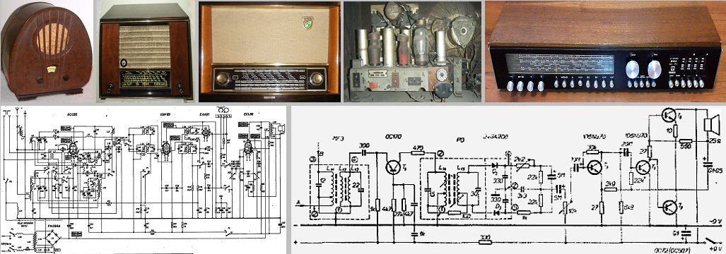
Radio receivers until approximately 1965 were equipped with
vacuum tubes, later mostly transistors, and most recently
integrated circuits, often with digitized electronics.
At our cottage in Konice, we gradually had several types
of now antique radio receivers (I
completely dismantled one of them as a 5-6 year old boy, so that
even an experienced radio technician could not repair it...). Later I liked to "hunt in the ether",
especially at night, when American and Chinese transmitters could
also be caught (although with fluctuations). I remember it fondly, it was nice and almost
"adventurous" ...
Author's
apology :
I wrote the passage about the transmission and
reception of radio waves here somewhat more technically focused
than is necessary for the physical explanation of
electrodynamics, gravity, space astrophysics. For me, it is a
kind of reminiscence of my school and grammar school years, when
electricity and radio engineering fascinated me. Already in the
8th and 9th grades of elementary school, I constructed two
radiotransmiters myself: for the range of about 0.5 - 30 MHz and
another around 70 - 100 MHz, equipped with EF22 and PL36 tubes.
And as a radio amateur, I tried to receive distant stations - DX (Distance reception at
X-distance, as large as possible; I even succeeded from China). I apologize to any readers
(otherwise oriented) for this subjective atypia and thank you for
your understanding...
Electromagnetic
waves of very high frequencies
To generate electromagnetic radiation of very high frequencies of
the order of GHz (e.g.
3-30 GHz) and
therefore short wavelengths of the order of centimeters (e.g. 10cm - 1cm), classic LC oscillators can no
longer be used, but instruments of high-frequency electronics. Oscillators
for these high frequencies are basically of two types :
-> Special vacuum tubes, magnetrons
and klystrons with resonant cavities (described in more detail in
§1.5, passage "Electrical power supply
of accelerators"). They are mainly used for large
high-frequency powers of the order of kilowatts to MW.
-> Special semiconductor components
with negative differential resistance, such as Gunn
diodes, tunnel diodes, IMPATT diodes (impact ionization avalanche diode). If such an element is
integrated into the circuit of a microwave resonant cavity and a
DC voltage U is applied (approx. 9V for a Gunn diode) to achieve the negative
resistance region, spontaneous oscillations begin to
occur (in the figure
on the left). The
frequency then depends on the size of the resonant cavity.
For conducting ultra-HF oscillating
voltage from the oscillator to the antenna, coaxial cables (where there are high losses) are no longer optimal, but waveguides
- metal tubes of rectangular or circular cross-section are often
used. When an electromagnetic wave strikes the conductive walls
of the tube obliquely, it is completely reflected from them. It
propagates in the longitudinal direction through the waveguide by
successive reflections. The superposition of the incident and
reflected waves creates a complex waves in the waveguide that has
a component of a progressive wave in the longitudinal direction
and a standing wave in the transverse direction.
In the simplest case, transmitting
antennas for centimeter radio waves can again be
ordinary wires or rod antennas with omnidirectional
effect. However, due to the short wavelengths, there is the
possibility of narrowly directional antennas in
the shape of funnels or paraboloids :
These very short waves propagate in a straight
line - only in direct visual visibility without obstacles,
there is no bending or reflection from the ionosphere. Receiving
antennas can again be wire (rod) without directional
effect, or directional parabolic.
For our astrophysical sciences, radio
telescopes (pictured
on the right) and
detection of microwave cosmic rays are important (§5.4, passage "Microwave relic radiation
- messenger of news about the early universe").
For even higher frequencies, in the infrared,
visible and UV radiation range, no electronic
oscillators and antennas work anymore, but this radiation is
created by vibrations of excited atoms and molecules in
substances. Special techniques are used here combining electronic
methods of atomic physics (including laser), with photomultipliers and semiconductor
photodiodes for detection and spectrometry of this
radiation.
And the highest frequencies and energies of X and gamma
radiation are already the domain of nuclear and
radiation physics (detailed discussion "Nuclear physics and physics of
ionizing radiation").
Electromagnetic waves are very
important in astrophysics, as they arise from a
variety of processes in the universe (in principle, almost all of them, even in the vicinity
of black holes). And
they allow us to investigate and indirectly "peek" into
these often extremely distant processes in the depths of the
universe - it is discussed in §1.1, passage "Electromagnetic radiation - the
basic source of information about the universe".
Plane electromagnetic
waves
In a plane wave propagating in the direction of the X axis, all
quantities are functions only t-x/c. If E = E
(t-x/c), then from Maxwell's equations (1.38) and (1.40) for r = 0, j = 0, it follows ¶B/¶t =
-rot E = (n°/c) ´ (dE/d(t-x/c))
= n°´ ¶E/¶t, so the relationship between electric
and magnetic field in an electromagnetic wave is
| B = n° x E / c , | (1.49) |
where n° is the unit vector in the direction of wave propagation ("x" indicates the vector product). That is, the vectors of electric and magnetic fields E and B are always perpendicular to each other and also to vector n° direction of propagation - electromagnetic waves are transverse. Since B = rot A, only the vector potential A is sufficient for the description of the plane wave, by which the fields E and B are determined by the relations
| E = A. x n° , B = (1/c) [(A. x n°) x n°] | (1.49 ') |
(the dot above A
means the time derivative: A.
= ¶A/¶t).
The simplest case of an electromagnetic
wave is a monochromatic wave, in which the field is a simple
harmonic function of time at each given point: A(t)r = const. = Ao(r) .cos(wt + a), a = a(r),
where w = 2p.f = 2p/T is
the circular frequency of the wave, a is a
constant phase shift. Size l = 2p c/w then represents the wavelength, ie
the distance that the wave travels in one period T (the
distance of the two nearest places with the same phase). In a
planar monochromatic wave, the field will be a harmonic function
of the argument t-x/c
A = Ao cos [w.(t - x/c) + a] ,
where Ao nor a does not depend on t nor x. By introducing a wave vector
| k = def ( w / c). n° | (1.50) |
a plane wave can be expressed in form
| A(r,t) = Ao cos (wt - k.r + a) | (1.51) |
valid for any direction of wave propagation (analogously for B and E). This expression for a monochromatic plane wave is often written in a imaginary complex form
| A = Re [Âo . e i(k.r - wt)] , | (1.51 ') |
where Âo = A .e i a is a constant complex vector; the fields E and B can be expressed similarly.
The
speed of propagation of an electromagnetic signal
The commotion - signal - in the electromagnetic
field therefore propagates in space with a finite speed c,
resulting from the retarded potentials (1.47a,b), which are
solutions to Maxwell's equations. We can measure the propagation
speed of electromagnetic signals in basically three environments
:
-> In a vacuum,
where it is the speed of light in a vacuum c =
299,792.458 km/s. - the maximum possible speed
of propagation of interactions in nature (§1.1, passage "Speed of light").
-> In a dielectric material
environment, where this speed c´= 1/Öem is somewhat smaller than c=1/Öeomo in a vacuum (§1.2, passage "Electromagnetic and optical
properties of substances"). In air (at normal pressure) it is 0.9997 c = 299,702 km/s, in water about 0.75 c = 225,000 km/s, in diamond only 0.413 c = 123,800 km/s.
-> In metal conductors
- electric wires - we measure the speed of movement of the electrical
signal along the conductor (we are no longer talking about
electromagnetic waves that do not penetrate inside the conductor), which is determined, in
addition to the speed of light in the given environment around
the conductor, also by the specific inductance and capacity
of the conductor . For a straight copper wire (cable thickness ~ 1 mm) approx. 0.65 c ~ 195,000 km/s was measured. It is worth
noting that the speed of propagation of an electromagnetic signal
in conductors somewhat depends on whether it is a
"bare" wire without insulation, or an insulated cable,
or coaxial.
In electronic circuits and
networks, the time delay of the signal is
important, given by dividing the length of the cable by the speed
of the signal. It limits the minimum width or maximum frequency
of pulses that networks and circuits are able to transmit and
process. In high-frequency electronics, phase shifts between
voltage and current and unwanted reflections and signal
interference occur in conductors. These effects of reflections
and signal interference can also significantly affect electronic
measurements of signal speed in conductors.
As
a result of these effects, there are above all artificially
higher - superluminal - measured signal propagation
speeds in electrical cables, from which sometimes rather
bombastic claims are derived such as "I measured the
superluminal speed of signal propagation in an electrical cable -
and thus disproved the theory of relativity! "...
Internal
angular momentum - spin - of electromagnetic waves
When turn of the coordinate system by an angle J around the direction of propagation n°
of plane electromagnetic waves, the field in the wave will be
transformed according to the law  ®
Â' = eiJ. Â; the electromagnetic wave is invariant
due to the rotation of an angle of 360° around the direction of
propagation. The symmetry properties of plane waves with
respect to rotation around the direction of propagation are
important in quantum physics, where they determine the spin of
the respective particles created by quantization of a given
field. At the classical level, spin is defined as
s = 360° / (angle of symmetry of a plane wave with respect to rotation about the direction of propagation) ;
the spin of the electromagnetic waves and their quanta - photons is therefore equal to s = 1 .
Orbital angular momentum
of an electromagnetic wave. Helically polarized radiation.
Momentum p is a quantity quantifying the
"intensity of motion" of an object of mass m
moving at speed v: p =
m.v. Angular momentum of momentum L
is then a quantity describing how this movement is oriented
relative to space - to reference points, usually to the origin of
the coordinates: L = r x p, where r
is the vector of the current distance of the particle from the
origin of the coordinates.
When a beam of electromagnetic radiation arrives, in addition to
energy, it usually also has a certain angular momentum relative
to the origin of the coordinate system. During interaction, it is
transferred together with energy (all or part of it) to a given
particle or system....
When electromagnetic waves are
emitted by a rotating source, this rotation
leaves specific traces on the structure of the emitted waves.
During the formation of a wave, the maximum and minimum E
and B shifts periodically in time
relative to each other during the rotation of the source, so the
phases of the wave - the alternation of maximum and minimum -
will shift as the wave propagates at speed c. The
wavefront takes on the helix shape of a spiral. A kind of "rotating,
twisting or spiral radiation" with specific
polarization properties is created. If it hits charged particles,
it causes, among other things, their rotation around the
direction of propagation of the beam, which can be considered as
a manifestation of the angular momentum of this
radiation. So it behaves like a wave with orbital angular
momentum.
In §4.4, the passage "Light propagation in the field of
a rotating black hole" it is discussed that a similar
situation can occur in rotating black holes, where the radiation
from the accretion disk can be spirally polarized in this way due
to the rotational deformation of spacetime.
Note: In laboratory optical experiments, this
light with helically rotating polarization is generated by
special rotating sources, cylindrical lenses, lasers, holograms,
and measured using spatial light modulators. For radio waves,
helical polarization can be achieved by a special spatial
configuration of antennas powered by phase-shifted alternating
signals, for sound waves analogously by speaker systems.
Gravitational waves arising in rotating systems of black holes or
neutron stars should also have a component of helical rotating
polarization (however, their measurement is complicated, so far
it has not been possible).
The general laws of wave origin and propagation in nature are discussed in §2.7, passage "Wave propagation - a general natural phenomenon".
Energy
of electromagnetic field
In electrostatics, it can be shown by simple considerations
(about the work needed to place the charges in a given
configuration) that the electrostatic energy of a system
of N charged bodies
ee = (1/2) a=1SN qa.ja = (1/2) nr.j dV = (1/8p) n E2 dV
can be expressed by the integral of the intensity of their common electric field, so that the electric field can be assigned the energy distributed with the density We = (1/8p) E2 in space. Similar considerations of labor required to produce the electric currents in the system of electrical circuits (against induced electromotive forces generated increase of the magnetic field), show that the energy of system this conductors
em = (1/2) a=1SN Ia.Fa = (1/2) nA.j dV = (1/8p) n B2 dV
is given by the volume integral of the induction vector B of the excited magnetic field and can be considered as the energy of this magnetic field distributed in space with density Wm = (1/8p) B2. The energy density in the electromagnetic field is then equal to the sum of the densities corresponding to the electric and magnetic components :
| Welmag = (1/8p) (E 2 + B 2 ) . | (1.52) |
It is clear that such an assignment of energy to the field is purely formal under Coulomb, Ampere, and Faraday's law, because it is just another description of the interaction energy in the idea of the instantaneous force action of charges and currents at a distance. However, the physical justification is given by the fact that the commotion in the electromagnetic field propagates at a finite speed. This final rate of propagation of changes in the field leads to the conclusion (repeat, see the argument in the introduction §2.8) that the electromagnetic field itself must actually contain energy (and momentum) that can flow from one place to another and perform work on electric charges and currents - changing to other forms of energy. The electromagnetic field is therefore not just a space in which electric and magnetic forces act, but is a separate physical reality - a specific form of matter.
By scalar multiplication of Maxwell's equation (1.38) by the field E and equation (1.40) by the field B and their addition we get the equation after adjustment
| ¶ [(E2 + B2)/8] / ¶t = - div [(c/4p).(E ´ B)] - j . E . | (1.53) |
Integration over some chosen spatial area V after the application of the Gauss theorem then gives
| |
(1.54) |
The left side represents the change in the energy of the electromagnetic field eelmag contained within the region V per unit time. The first integral on the right indicates the work that electric forces do with charges per unit time, or the change in kinetic energy ekin of charges per unit time (magnetic forces with charges do no work and therefore do not change their kinetic energy). Equation (1.54) thus expresses the law of conservation of energy in the electromagnetic field: the electromagnetic energy contained in the spatial region V decreases on the one hand by mechanical work performed by electric forces with charges inside the region V , on the other hand by energy transmitted (radiated) by the field from the area V through the bounding surface S = ¶V to the outer space. Equation (1.54) can also be written in the form
| |
(1.54 ') |
whereby a decrease in total energy of the electromagnetic field and the charged particles in the volume V per unit time is equal to the flux vector (c/4p). (E x B) by the surface S surrounding region V. Therefore the vector
| P = (c / 4p ). ( E x B ) | (1.55) |
called the Poynting
vector, represents the energy passing through a unit of area
per unit of time, or it is a vector of the flux density of
electromagnetic energy in space. When integrating in (1.54)
over the whole space, when the bounding surface S is
infinitely spaced and the field on it is equal to zero, it
expresses equation (1.54), resp. (1.54'), simply the law of
conservation of the sum of the total energy of the
electromagnetic field and the kinetic energy of all charges.
Similarly, it can be shown that the
electromagnetic field has momentum p given by the integral
| p = ò (1/4p c). ( E x B ) dV , |
so the momentum of the
volume unit of the electromagnetic field is equal to P/c2 .
Energy transmitted by
electromagnetic waves
Electromagnetic waves carry a certain part of the energy from the
source system into the surrounding space. At a sufficiently large
distance - in the wave zone - they already exist independently,
without being connected to the original source, which is then no
longer affected by whether the wave has transmitted its energy
somewhere. The electromagnetic wave itself contains energy
regardless of whether it is absorbed or not. When a wave
encounters a system of electric charges, its oscillating electric
and magnetic fields can exert forces and move these charges -
perform work, transmit energy. A greater or lesser part
of the wave's energy is thereby absorbed, the intensity decreases
and possibly the remaining part travels further.
The greater the intensity of the
electric E and magnetic B
fields - the amplitude of the wave - the greater the
energy the wave carries and the greater the effect it can have on
the electric charges. The energy flow density in a plane
electromagnetic wave is, with respect to (1.49), equal
| P = (c/4p) ( E x B ) = (c/4p) E2.n° = (c/4p) B2.n° , |
which with respect to (1.52) is related to the energy density Welmag by the relation P = c. Welmag . n°, from which it can also be seen that both the field and energy propagates in the wave at the speed of light.
The density of electric energy in an electric field is We = (1/2)eo E2. The density of magnetic energy in a magnetic field is Wm = B2/(2mo). The energy at any place and time in an electromagnetic wave is given by the sum of the energies of the electric and magnetic fields, i.e. for densities :
Welmag = We + Wm = 1/2 eo E2 + 1/2mo.B2 .
In an electromagnetic wave, E and B are related by the relation E = c.B, the speed of light in a vacuum is 1/Ö(e0.m0). So in an electromagnetic wave, the electric and magnetic energy densities are related :
| We = 1/2 eo E2 = 1/2 eo B2 c2 = 1/2 eo B2 /(e0.m0) = 1/2mo.B2 = Wm , | (1.56) - SI |
i.e. the magnetic energy density Wm and the electric energy density We are the same here, despite the fact that a changing electric field generally produces only a weak magnetic field. The total energy of the wave is then W = We + Wm = eo E2 . The intensity of the electromagnetic wave, which is the energy passing through a unit area (perpendicular to the direction of propagation) per unit time, is then IW = c.eo.E2 .
Electromagnetic energy
radiation
Let us have a system of moving electric charges concentrated in
some limited spatial area (Fig.1.4). If we place the origin of
coordinates somewhere into the system of charges, then the study
of the field at large distances R >> L, where L is
the characteristic dimension of the system will place all of the
source system at about the same distance R as the origin
of the coordinates. Distances |R - r| of the
individual points r' of the source from the investigated
distant point R is approximately equal to |R - r'|
@ R - R°. r', where R°
is a unit vector pointing from the origin O to the
investigated point, so that the retarded potential can be written
in the form
j(R,t) = (1/R). n r(r', t - R/c + R°.r'/c) dV' , A(R,t) = (1/R). n j(r', t - R/c + R°.r'/c) dV' .
The retardation time
thus consists of two different parts. The first part R/c
determines the external retardation, ie the time required for the
changes in the electromagnetic field to exceed the distance from
the origin of the coordinates, or from the source system, to the
distant observation point. The second part equal to - R°.
r'/c characterizes the internal retardation, ie the time
of propagation of the disturbance in the field within the source
system.
If the charge distribution in the system changes slowly enough,
internal retardation can be neglected. For this, it is sufficient
that the characteristic time T, during which the charge
distribution changes appreciably, satisfies the condition T
>> L/c. Since c.T is the wavelength l of electromagnetic waves emitted
by the system, the condition of negligibility of internal
retardation can also be written in the form L << l, ie the dimensions of the system must be
small in comparison with the length of the emitted waves. The
characteristic time T changes in the distribution of
charges is related to the average velocity v of charges
rounds following equation: T »
L/v, so that
neglecting retardation it is necessary to apply v«c, i.e. the
speed of motion of charges must be small compared to the speed of
light. If internal retardation is neglected, the potentials are
equal at great distances from the source system
j(R,t) = (1/R). n r(r', t - R/c) dV' , A(R,t) = (1/R). n j(r', t - R/c) dV' .
At these distances large in comparison with both the dimensions of the source system and the length of the radiated waves - in the wave zone - it is possible to consider the variable field component as a plane wave within small areas of space. It is therefore sufficient to determine the vector potential A = (1/cR). n r.v dV' = (1/cR)a=1SNqava = (1/cR) (d/dt)a=1SNqar'a , i.e.
| A(R , t) = (1 / c.R). d. (t- R/c) , | (1.58) |
where d º S qa ra is the electric dipole moment of the system as it was at time t-R/c. The electric and magnetic fields are then, according to (1.49), equal
| E(R,t) = (1/c2R) [ (d.. x R°) ´ R°] , B(R,t) = (1/c2R) (d.. x R°) , | (1.59) |
where the dipole moment d is again taken at the moment t-R/c (dots above d mean the derivative according to time).
The flow of electromagnetic energy in the wave zone, ie the intensity of electromagnetic radiation, is expressed by the Poynting vector according to (1.57)
| P = (c/4p) (E´B) = (1/4pc3R2) (d..xR°)2 = (d.. 2/4pc3R2) sin2J . R° , | (1.60) |
where J is the angle between the directions of the vectors d.. and R (if we use polar coordinates - Fig.1.4b). The angular distribution of the intensity of the electric dipole radiation is given by the coefficient sin2J , the corresponding directional diagram is in Fig.1.4c. The total energy radiated by the system per unit time (ie radiated power) I = dE/dt is then given by the flow of energy over the entire spherical surface R = const. :
 |
(1.61) |
If the source system consists of only one accelerating charge q, is d.. = q. r.. = q. a, and the radiated power is equal to
| I º dE / dt = (2.q2 / 3c3 ). a 2 . | (1.61 ') |
This radiation law was derived in 1899 by the Irish physicist J.Larmor. In addition, in the system of SI units, there is a coefficient k = 1/ (4p eo) present in Coulomb's law.

Fig.1.4. Electromagnetic field of an island system of moving
electric charges.
a ) The field excited by a system of moving electric
charges is given not by an instantaneous but by a retarded
distribution and movement of the charges.
b ) At a great distance from the source system (in the
wave zone), the variable component of the field is given by the
second time derivative of the dipole moment of the system d..
and has the character of electromagnetic waves carrying the
kinetic energy of the source into space.
c ) Directional diagram of electric dipole radiation.
Relationships (1.58) to (1.61) for the field and radiation of the island system of electric charges in the wave zone were obtained in the first order approximation in the ratio L/l (higher order members were neglected), which led to the application of only the dipole moment of the system. In the general case, however, it is necessary to take into account other members in the development of the potential according to powers L/l, which leads to the fact that the total intensity of electromagnetic radiation of a system of moving charges is given by time derivatives of individual multipole moments of charge distribution. In addition to the dipole moment is usually the most radiation involved the quadrupole moment Kab = n r.(3xaxb - dab.r2) dV and possibly magnetic dipole moment m = (1/2c) n r.(rxv)dV, which contribute to radiation according to a known relationship (see eg [166])
| (1.62) |
If the properties of the source system are such that d.. = 0 (this is the case, for example, in a system composed of bodies with the same specific charge q/m), dipole radiation does not occur. In such cases, only radiation caused by other members in the development of the potential according to powers of L/l , ie radiation of higher multipoles, is applied.
Electrodynamics thus
comes to the general conclusion that with each accelerated
(uneven) movement of electric charges, electromagnetic waves
are emitted, which carry part of their kinetic
energy into space *). In §2.7 we will see that the general
theory of relativity arrives at essentially the same conclusion -
the emission of gravitational waves during the accelerated motion
of gravitational bodies, although the properties of gravitational
waves differ from the properties of electromagnetic waves in some
respects (above all, they are many times weaker).
*) This phenomenon
plays an important role in atomic physics for the structure of
the atomic shell and the formation of radiation during its
deexcitation (see §1.1 "Atoms
and atomic nuclei" of the book "Nuclear Physics and Physics of
Ionizing Radiation"). Furthermore, in nuclear physics and
physics of ionizing radiation. Particularly fast-flying electrons
are sharply braked when interacting with the
material environment, so that according to the relation (1.61´)
they emit relatively intense electromagnetic radiation -
so-called braking radiation. Braking radiation
finds significant use in the excitation of X-rays
by the impact of electrically accelerated electrons on the anode
in X-rays tubes - see §3.2 "X-ray diagnostics", or in the excitation of
hard g- radiation by the
impact of high-energy electrons from betatron or linear
accelerator on a suitable target (see §1.5 "Elementary
particles", the section "Charged Particle Accelerators" of the same publication) .
We investigated the variable electromagnetic fields excited by a system of moving charges in the wave zone, ie at sufficiently large distances from the source system, and we calculated the radiated energy using the Poynting vector. Analysis of the electromagnetic field at short distances then shows that a small variable component of the electric field with a phase different from the main variable component is generated inside and near the source system. In the third order approximation, this term is equal
Ere = (2 / 3c 3 ) d ... .
In the source system, therefore, each charge q will be subjected to a certain additional force "reaction" fre = q. Ere acting per unit time of work fre.v so that the total work performed by this field with all charges of the system system comes out A re = (2/3c3) d... S qava = (2/3c3) d... .d., which when averaged over time (over several periods T) gives
A re = - (2 / 3 c3 ) d.. 2 .
It can be seen that this
additional field component causes a corresponding braking
of the charge movements in the source by the back reaction of the
emitted waves, in full energy agreement with the formula (1.61)
obtained by the analysis of the field in the far wave zone. Such
an analysis is of great importance for gravitational waves, where
the calculation of energy in the wave zone is not nearly as clear
and unambiguous as in electrodynamics - we will see this in §2.8
"Specific properties of
gravitational energy".
Equation of motion m. v = q. E
+ (q/c). ( v x B ) charged particles in
the electromagnetic field under the influence of the Lorentz
force (1.30) is therefore necessary to supplement the braking
action of electromagnetic radiation :
| m .v = q.E + (q/c) (v x B) + (2q2/3c3) v.. ; | (1.63) |
this equation is
applicable when the velocity is small compared to the speed of
light and the braking force is significantly smaller than the
Lorentz force acting on the charge of the external field E
and B.
Further details on the properties of
the electromagnetic field and their applications can be found in
the relevant literature; from review momographies we can mention
eg [235], [264], [206].
E
t h e r
Electromagnetic fields in the past have been considered as a
manifestation of certain types of ether motion *). Some
(electrically charged) bodies set this ether in motion, which
propagates in it at a finite speed and is passed on to other
bodies. However, such an ether would have to have very unusual
physical properties. In order for electromagnetic waves to
propagate in it, which are transverse, it would have to have some
properties of a solid body. And the mechanical model of the ether
is no longer compatible with the experimentally determined
constant of the speed of light in all inertial systems. Attempts
to reconcile this fact with the ether model did not lead to
success (for
example, the assumption of "entrainment of the ether"
by the movement of the Earth failed to confront the observed
aberration of light from the constellations). Therefore, the idea of ether was
abandoned and it was realized that the carrier of the
electromagnetic field is the space itself . A. Einstein
then completed this concept in a special theory of relativity by
concluding that the stability of the speed of light is a
reflection of the connection between space and time.
Electromagnetism thus played an important heuristic role in
revealing the deeper and more general laws of nature - the laws
of relativistic physics .
*) Ether :
According to ancient Greek philosophers and naturalists
(especially Aristotles), the "heavenly" space - the
universe - was filled with a hypothetical ubiquitous invisible
subtle substance called ether (Greek aithér,
Lat. ether = bright light, sky, upper layers of air).
They imagined the ether as a flexible, transparent liquid,
perfectly permeable without friction, unweightable,
indestructible. Together with the other elements "earth,
water, air, fire" as the "fifth element",
which does not act on the earth's surface, but in the celestial
spheres. All celestial bodies, stars, planets, the Sun are
created from the ether. Ether transmits light and heat from the
Sun and light from stars and planets.
Note:
In chemistry, aether is called a volatile
organic solvent.
19th century physics she took it for
granted that every wave could propagate only in the flexible
material (matter) medium whose oscillating motion created it. It
is difficult to imagine sea waves without water or sound without
air (or other flexible acoustic environment of gaseous, liquid or
solid phase - see the well-known elementary experiment with an
alarm clock or a bell under the recipient of the vacuum pump).
When it was discovered that light and other electromagnetic waves
propagate not only in air and other optical media environments,
but also in a vacuum, a problem arose in the environment
or medium in which electromagnetic waves propagate. So once again
revived the idea of ether - universal all-
pervading "substances", filling all space and
penetrating all matter (just as water penetrates the meshes of a
fishing net towed behind a boat). This ether creates an
environment for the propagation of light, heat and other
electromagnetic waves; it is also a carrier of gravity. Since the
ether did not manifest itself in any other physical and chemical
phenomena, it was judged to be translucent, unweightable,
perfectly permeable without friction, and had no chemical
properties. A substance with such conflicting properties was
practically undetectable experimentally.
One could only study how the
penetration of ether affects the speed of light
under different configurations of the state of motion of the
light source and the observer. Maxwell himself has already
designed an experiment using the motion of the Earth: light
moving with the ether in the same direction as the Earth orbits
the Sun must have a slightly different speed than light that
propagates perpendicular to this motion or in the opposite
direction. be about 10-7. Maxwell did not see the result of this
experiment; up to 8 years after his death, in 1887, A.Michelson
and E.Morley made this measurement by interfering with the rays
of monochromatic light reflected by two mirrors in the horizontal
and vertical directions, while the whole interference device on
the floating plate could be rotated. The result was that no
difference was measured in the speed of light in both
directions, seemed unexpected and paradoxical at the time.
However, the negative result of this experiment was confirmed by
other measurements. No ad hoc hypotheses, such as ether
entrainment (the ether is drawn along with the earth's surface,
so its position relative to the interferometer) has not been
confirmed. In contrast, the negative result of Michesson's and
Morley's experiment was explained by the Lorentz contraction
hypothesis, according to which the dimensions of all
bodies in the direction of their velocity v are shortened
in the ratio 1/ Ö (1-v2/c2). Einstein then gave a definitive and
universal explanation in his special theory of relativity,
according to which the speed of light (in vacuum) is the same in
all moving conditions and in all directions. The idea of the
ether was thus definitively abandoned, replaced
by the properties of empty space itself, connected with time into
a single space-time continuum. Nevertheless, in
the field of radio applications of electromagnetic waves, the
terms "transmit to ether" or "receive
from ether" are often used.
However, after the creation of
general relativity, Einstein recognized that the role of the
earlier static ether is equivalently played by the space-time
continuum, which is dynamic and is described by the metric tensor
field gik .
Nonlinear electrodynamics
?
At all the intensities we observe in nature and in the
laboratory, the electric and magnetic fields in the vacuum appear
to us to be linear - the principle of
superposition applies exactly to the values of
intensities E and B, as well as
to potentials.
At the end of the following §1.6 "Four-Dimensional
Spacetime and
Special Theory of Relativity", passage "Nonlinear Electrodynamics", the possibilities of how
an extremely strong electromagnetic field could behave in a non-linear
manner even in a vacuum will be discussed.
| 1.4. Analogy between
gravity and electrostatics |
1.6. Four-dimensional
spacetime and special theory of relativity |
| Gravity, black holes and space-time physics : | ||
| Gravity in physics | General theory of relativity | Geometry and topology |
| Black holes | Relativistic cosmology | Unitary field theory |
| Anthropic principle or cosmic God | ||
| Nuclear physics and physics of ionizing radiation | ||
| AstroNuclPhysics ® Nuclear Physics - Astrophysics - Cosmology - Philosophy | ||